# GreptimeDB Documentation
> GreptimeDB is an open-source observability database for metrics, logs, traces, and wide events. Drop-in replacement for Prometheus, Loki & Elasticsearch, or the single backend for OpenTelemetry.
This file contains all documentation content in a single document following the llmstxt.org standard.
## GreptimeDB
# Introduction
**GreptimeDB** is an open-source observability database that handles metrics, logs, and traces in one engine. Use it as the single OpenTelemetry backend — replacing Prometheus, Loki, and Elasticsearch with one database built on object storage. Query with [SQL](/user-guide/query-data/sql.md) and [PromQL](/user-guide/query-data/promql.md), scale without pain, cut costs up to 50x.
## Why GreptimeDB
**Replace three systems with one.** Most teams run Prometheus for metrics, Loki or ELK for logs, and Elasticsearch or Tempo for traces — three systems, three query languages, three sets of operational overhead. GreptimeDB unifies all three in a single engine with native OpenTelemetry support.
**Cut costs up to 50x.** Object storage (S3, Azure Blob, GCS) as primary data store with compute-storage separation. Compute nodes scale independently. Written in Rust with columnar storage and advanced compression for maximum efficiency.
**Drop-in compatible.** [PromQL](/user-guide/query-data/promql.md), [Prometheus remote write](/user-guide/ingest-data/for-observability/prometheus.md), [Jaeger](/user-guide/query-data/jaeger.md), [MySQL](/user-guide/protocols/mysql.md), [PostgreSQL](/user-guide/protocols/postgresql.md) protocols — migrate without rewriting queries. [SQL](/user-guide/query-data/sql.md) + [PromQL](/user-guide/query-data/promql.md) dual query capability means one database replaces your metrics store + data warehouse combo.
Learn more in [Why GreptimeDB](/user-guide/concepts/why-greptimedb.md) and [Observability 2.0](/user-guide/concepts/observability-2.md).
Before getting started, please read the following documents that include instructions for setting up, fundamental concepts, architectural designs, and tutorials:
- [Getting Started][1]: Provides an introduction to GreptimeDB for those who are new to it, including installation and database operations.
- [For AI Agents][8]: Use GreptimeDB with AI agents via the MCP Server, Skills, and machine-readable docs.
- [User Guide][2]: For application developers to use GreptimeDB or build custom integration.
- [Contributor Guide][3]: For contributors interested in learning more about the technical details and enhancing GreptimeDB.
- [Roadmap][7]: The latest GreptimeDB roadmap.
- [Release Notes][4]: Presents all historical version release notes.
- [FAQ][5]: Provides answers to the most frequently asked questions.
[1]: ./getting-started/overview.md
[8]: ./faq-and-others/vibecoding.md
[2]: ./user-guide/overview.md
[3]: ./contributor-guide/overview.md
[4]: /release-notes
[5]: ./faq-and-others/faq.md
[7]: https://greptime.com/blogs/2026-02-11-greptimedb-roadmap-2026
---
## GreptimeDB Cluster
The GreptimeDB cluster can run in cluster mode to scale horizontally.
## Deploy the GreptimeDB cluster in Kubernetes
For production environments, we recommend deploying the GreptimeDB cluster in Kubernetes. Please refer to [Deploy on Kubernetes](/user-guide/deployments-administration/deploy-on-kubernetes/overview.md).
## Use Docker Compose
:::tip NOTE
Although Docker Compose is a convenient way to run the GreptimeDB cluster, it is only for development and testing purposes.
For production environments or benchmarking, we recommend using Kubernetes.
:::
### Prerequisites
Using Docker Compose is the easiest way to run the GreptimeDB cluster. Before starting, make sure you have already installed the Docker.
### Step1: Download the YAML file for Docker Compose
```
wget https://raw.githubusercontent.com/GreptimeTeam/greptimedb/v1.0.2/docker/docker-compose/cluster-with-etcd.yaml
```
### Step2: Start the cluster
```
GREPTIMEDB_VERSION=v1.0.2 \
docker compose -f ./cluster-with-etcd.yaml up
```
If the cluster starts successfully, it will listen on 4000-4003. , you can access the cluster by referencing the [Quick Start](../quick-start.md).
### Clean up
You can use the following command to stop the cluster:
```
docker compose -f ./cluster-with-etcd.yaml down
```
By default, the data will be stored in `./greptimedb-cluster-docker-compose`. You also can remove the data directory if you want to clean up the data.
## Next Steps
Learn how to write data to GreptimeDB in [Quick Start](../quick-start.md).
---
## GreptimeDB Dashboard
Visualization plays a crucial role in effectively utilizing time series data. To help users leverage the various features of GreptimeDB, Greptime offers a simple [dashboard](https://github.com/GreptimeTeam/dashboard).
The Dashboard is embedded into GreptimeDB's binary since GreptimeDB v0.2.0. After starting [GreptimeDB Standalone](greptimedb-standalone.md) or [GreptimeDB Cluster](greptimedb-cluster.md), the dashboard can be accessed via the HTTP endpoint `http://localhost:4000/dashboard`. The dashboard supports multiple query languages, including [SQL queries](/user-guide/query-data/sql.md), and [PromQL queries](/user-guide/query-data/promql.md).
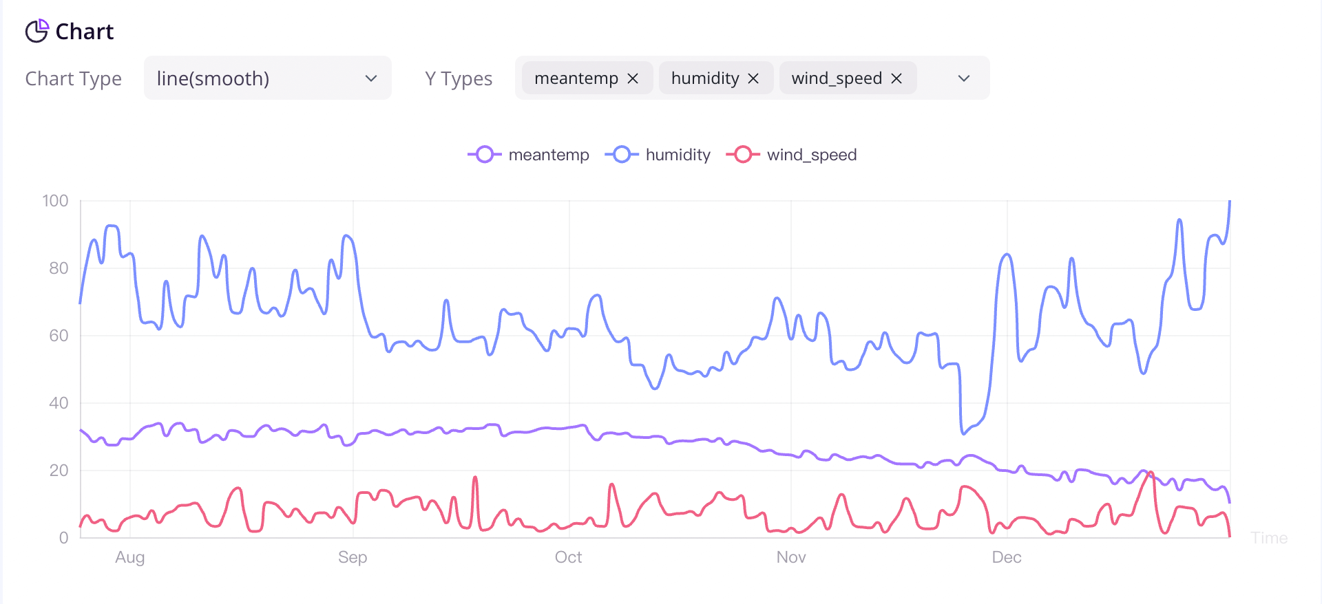
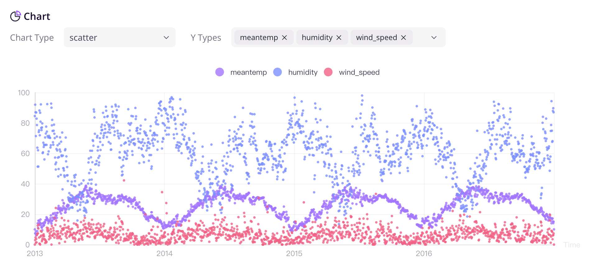
We offer various chart types to choose from based on different scenarios. The charts become more informative when you have sufficient data.
We are committed to the ongoing development and iteration of this open-source project, and we plan to expand the application of time series data in monitoring, analysis, and other relevant fields in the future.
---
## GreptimeDB Standalone
We use the simplest configuration for you to get started. For a comprehensive list of configurations available in GreptimeDB, see the [configuration documentation](/user-guide/deployments-administration/configuration.md).
## Deploy the GreptimeDB standalone in Kubernetes
For production environments, we recommend deploying the GreptimeDB standalone in Kubernetes. Please refer to [Deploy on Kubernetes](/user-guide/deployments-administration/deploy-on-kubernetes/overview.md).
## Binary
### Download from website
You can try out GreptimeDB by downloading the latest stable build releases from the [Download page](https://greptime.com/download).
### Linux and macOS
For Linux and macOS users, you can download the latest build of the `greptime` binary by using the following commands:
```shell
curl -fsSL \
https://raw.githubusercontent.com/greptimeteam/greptimedb/main/scripts/install.sh | sh -s v1.0.2
```
Once the download is completed, the binary file `greptime` will be stored in your current directory.
You can run GreptimeDB in the standalone mode:
```shell
./greptime standalone start
```
### Windows
If you have WSL([Windows Subsystem for Linux](https://learn.microsoft.com/en-us/windows/wsl/about)) enabled, you can launch a latest Ubuntu and run GreptimeDB like above!
Otherwise please download the GreptimeDB binary for Windows at our [official site](https://greptime.com/resources), and unzip the downloaded artifact.
To run GreptimeDB in standalone mode, open a terminal (like Powershell) at the directory where the GreptimeDB binary locates, and execute:
```shell
.\greptime standalone start
```
## Docker
Make sure the [Docker](https://www.docker.com/) is already installed. If not, you can follow the official [documents](https://www.docker.com/get-started/) to install Docker.
```shell
docker run -p 127.0.0.1:4000-4003:4000-4003 \
-v "$(pwd)/greptimedb_data:/greptimedb_data" \
--name greptime --rm \
greptime/greptimedb:v1.0.2 standalone start \
--http-addr 0.0.0.0:4000 \
--rpc-bind-addr 0.0.0.0:4001 \
--mysql-addr 0.0.0.0:4002 \
--postgres-addr 0.0.0.0:4003
```
:::tip NOTE
To avoid accidentally exit the Docker container, you may want to run it in the "detached" mode: add the `-d` flag to
the `docker run` command.
:::
The data will be stored in the `greptimedb_data/` directory in your current directory.
If you want to use another version of GreptimeDB's image, you can download it from our [GreptimeDB Dockerhub](https://hub.docker.com/r/greptime/greptimedb). In particular, we support GreptimeDB based on CentOS, and you can try image `greptime/greptimedb-centos`.
:::tip NOTE
If you are using a Docker version lower than [v23.0](https://docs.docker.com/engine/release-notes/23.0/), you may experience problems with insufficient permissions when trying to run the command above, due to a [bug](https://github.com/moby/moby/pull/42681) in the older version of Docker Engine.
You can:
1. Set `--security-opt seccomp=unconfined`, for example:
```shell
docker run --security-opt seccomp=unconfined -p 4000-4003:4000-4003 \
-v "$(pwd)/greptimedb_data:/greptimedb_data" \
--name greptime --rm \
greptime/greptimedb:v1.0.2 standalone start \
--http-addr 0.0.0.0:4000 \
--rpc-bind-addr 0.0.0.0:4001 \
--mysql-addr 0.0.0.0:4002 \
--postgres-addr 0.0.0.0:4003
```
2. Upgrade the Docker version to v23.0.0 or higher;
:::
## Binding address
GreptimeDB binds to `127.0.0.1` by default. If you need to accept connections from other addresses, you can start with the following parameters.
> :::danger Warning
> If the computer running GreptimeDB is directly exposed to the internet, binding to `0.0.0.0` is dangerous and will expose the instance to everybody on the internet.
```shell
./greptime standalone start \
--http-addr 0.0.0.0:4000 \
--rpc-bind-addr 0.0.0.0:4001 \
--mysql-addr 0.0.0.0:4002 \
--postgres-addr 0.0.0.0:4003
```
```shell
docker run -p 0.0.0.0:4000-4003:4000-4003 \
-v "$(pwd)/greptimedb_data:/greptimedb_data" \
--name greptime --rm \
greptime/greptimedb:v1.0.2 standalone start \
--http-addr 0.0.0.0:4000 \
--rpc-bind-addr 0.0.0.0:4001 \
--mysql-addr 0.0.0.0:4002 \
--postgres-addr 0.0.0.0:4003
```
You can also refer to the [Configuration](/user-guide/deployments-administration/configuration.md) document to modify the bind address in the configuration file.
## Next Steps
Learn how to write data to GreptimeDB in the [Quick Start](../quick-start.md).
---
## GreptimeDB Installation Overview
# Installation
Follow these instructions to install GreptimeDB:
- [GreptimeDB Standalone](greptimedb-standalone.md) runs as a standalone system in a single process.
- [GreptimeDB Cluster](greptimedb-cluster.md) runs as a distributed, clustered time series database.
## Check database health
After starting GreptimeDB, you can check its status to ensure it is running.
```shell
curl http://localhost:4000/health
```
If the GreptimeDB instance is running healthily, you will see the following response:
```json
{}
```
## Next steps
- [Quick Start](/getting-started/quick-start.md): Ingest and query data in GreptimeDB using MySQL or PostgreSQL clients.
---
## GreptimeDB Getting Started Overview
# Getting Started
> **AGENT ONBOARDING:** Read https://docs.greptime.com/SKILL.md and follow the instructions to use GreptimeDB with your AI agent — deploy, configure, ingest, and query.
Get started with GreptimeDB quickly by following these steps:
- [Installation](./installation/overview.md): Learn how to install GreptimeDB as a standalone or cluster.
- [Quick Start](./quick-start.md): Get started with GreptimeDB using your preferred protocols or languages.
- [For AI Agents](../faq-and-others/vibecoding.md): Use GreptimeDB with AI agents via the MCP Server, Skills, and machine-readable docs.
---
## GreptimeDB Getting Started Quick Start
# Quick Start
Before proceeding, please ensure you have [installed GreptimeDB](./installation/overview.md).
This guide uses SQL to walk you through GreptimeDB's core capabilities — from ingestion to cross-signal correlation across metrics, logs, and traces. SQL is also GreptimeDB's management interface for creating tables, setting TTL policies, and configuring indexes.
:::tip Already running Prometheus, OpenTelemetry, Loki or ES?
You can start ingesting data immediately using your existing tools — no schema creation needed (GreptimeDB [creates tables automatically](/user-guide/ingest-data/overview.md#automatic-schema-generation)):
- [Prometheus Remote Write](/user-guide/ingest-data/for-observability/prometheus.md)
- [OpenTelemetry (OTLP)](/user-guide/ingest-data/for-observability/opentelemetry.md)
- [Loki Protocol](/user-guide/ingest-data/for-observability/loki.md)
- [Elasticsearch](/user-guide/ingest-data/for-observability/elasticsearch/)
Continue with this guide to see what you can do with the data once it's in.
:::
**You'll learn (10–15 minutes):**
- Connect to GreptimeDB and create metrics, logs, and traces tables
- Query and aggregate data with SQL
- Search logs by keyword with full-text index
- Compute p95 latency in time windows using range queries
- **Correlate metrics, logs, and traces in a single query**
- Combine SQL and PromQL
## Connect to GreptimeDB
GreptimeDB supports [multiple protocols](/user-guide/protocols/overview.md) for interacting with the database. In this guide, we use SQL for simplicity.
If your GreptimeDB instance is running on `127.0.0.1` with the MySQL client default port `4002` or the PostgreSQL client default port `4003`, connect using:
```shell
mysql -h 127.0.0.1 -P 4002
```
Or
```shell
psql -h 127.0.0.1 -p 4003 -d public
```
You can also use the built-in Dashboard at `http://127.0.0.1:4000/dashboard` to run all the SQL queries in this guide.
By default, GreptimeDB does not have [authentication](/user-guide/deployments-administration/authentication/overview.md) enabled. You can connect without providing a username and password.
## Create tables
We'll create three tables to simulate a real scenario: gRPC latency metrics, application logs, and request traces. Two application servers, `host1` and `host2`, are recording data. Starting from `2024-07-11 20:00:10`, `host1` begins experiencing issues.
### Metrics table
```sql
-- Metrics: gRPC call latency in milliseconds
CREATE TABLE grpc_latencies (
ts TIMESTAMP TIME INDEX,
host STRING,
method_name STRING,
latency DOUBLE,
PRIMARY KEY (host, method_name)
);
```
- `ts`: Timestamp when the metric was collected (the [time index](/user-guide/concepts/data-model.md)).
- `host` and `method_name`: [Tag](/user-guide/concepts/data-model.md) columns identifying the time series.
- `latency`: [Field](/user-guide/concepts/data-model.md) column containing the actual measurement.
### Logs table
```sql
-- Logs: application error logs
CREATE TABLE app_logs (
ts TIMESTAMP TIME INDEX,
host STRING,
api_path STRING,
log_level STRING,
log_msg STRING FULLTEXT INDEX WITH('case_sensitive' = 'false'),
PRIMARY KEY (host, log_level)
) WITH ('append_mode'='true');
```
- `log_msg` enables [full-text index](/user-guide/manage-data/data-index.md#fulltext-index) for keyword search.
- [`append_mode`](/user-guide/deployments-administration/performance-tuning/design-table.md#when-to-use-append-only-tables) optimizes for log workloads (no deduplication overhead).
### Traces table
```sql
-- Traces: request spans
CREATE TABLE traces (
ts TIMESTAMP TIME INDEX,
trace_id STRING SKIPPING INDEX,
span_id STRING,
parent_span_id STRING,
service_name STRING,
operation STRING,
duration DOUBLE,
status_code INT,
PRIMARY KEY (service_name)
) WITH ('append_mode'='true');
```
For high-cardinality `trace_id`s, we have enabled the [skip index](/user-guide/manage-data/data-index.md#skipping-index).
:::tip
We use SQL to ingest data below, so we create the tables manually. However, GreptimeDB is [schemaless](/user-guide/ingest-data/overview.md#automatic-schema-generation) — when using protocols like OpenTelemetry, Prometheus Remote Write, or InfluxDB Line Protocol, tables are created automatically.
:::
## Write data
Let's insert sample data simulating the scenario. Before `20:00:10`, both hosts are normal. After `20:00:10`, `host1` starts experiencing latency spikes.
### Normal period (before 20:00:10)
```sql
INSERT INTO grpc_latencies (ts, host, method_name, latency) VALUES
('2024-07-11 20:00:06', 'host1', 'GetUser', 103.0),
('2024-07-11 20:00:06', 'host2', 'GetUser', 113.0),
('2024-07-11 20:00:07', 'host1', 'GetUser', 103.5),
('2024-07-11 20:00:07', 'host2', 'GetUser', 107.0),
('2024-07-11 20:00:08', 'host1', 'GetUser', 104.0),
('2024-07-11 20:00:08', 'host2', 'GetUser', 96.0),
('2024-07-11 20:00:09', 'host1', 'GetUser', 104.5),
('2024-07-11 20:00:09', 'host2', 'GetUser', 114.0);
```
### Anomalous period (after 20:00:10)
`host1`'s latency becomes unstable with spikes up to several thousand milliseconds:
Click to expand INSERT statements
```sql
INSERT INTO grpc_latencies (ts, host, method_name, latency) VALUES
('2024-07-11 20:00:10', 'host1', 'GetUser', 150.0),
('2024-07-11 20:00:10', 'host2', 'GetUser', 110.0),
('2024-07-11 20:00:11', 'host1', 'GetUser', 200.0),
('2024-07-11 20:00:11', 'host2', 'GetUser', 102.0),
('2024-07-11 20:00:12', 'host1', 'GetUser', 1000.0),
('2024-07-11 20:00:12', 'host2', 'GetUser', 108.0),
('2024-07-11 20:00:13', 'host1', 'GetUser', 80.0),
('2024-07-11 20:00:13', 'host2', 'GetUser', 111.0),
('2024-07-11 20:00:14', 'host1', 'GetUser', 4200.0),
('2024-07-11 20:00:14', 'host2', 'GetUser', 95.0),
('2024-07-11 20:00:15', 'host1', 'GetUser', 90.0),
('2024-07-11 20:00:15', 'host2', 'GetUser', 115.0),
('2024-07-11 20:00:16', 'host1', 'GetUser', 3000.0),
('2024-07-11 20:00:16', 'host2', 'GetUser', 95.0),
('2024-07-11 20:00:17', 'host1', 'GetUser', 320.0),
('2024-07-11 20:00:17', 'host2', 'GetUser', 115.0),
('2024-07-11 20:00:18', 'host1', 'GetUser', 3500.0),
('2024-07-11 20:00:18', 'host2', 'GetUser', 95.0),
('2024-07-11 20:00:19', 'host1', 'GetUser', 100.0),
('2024-07-11 20:00:19', 'host2', 'GetUser', 115.0),
('2024-07-11 20:00:20', 'host1', 'GetUser', 2500.0),
('2024-07-11 20:00:20', 'host2', 'GetUser', 95.0);
```
### Error logs during the anomaly
```sql
INSERT INTO app_logs (ts, host, api_path, log_level, log_msg) VALUES
('2024-07-11 20:00:10', 'host1', '/api/v1/resource', 'ERROR', 'Connection timeout'),
('2024-07-11 20:00:10', 'host1', '/api/v1/billings', 'ERROR', 'Connection timeout'),
('2024-07-11 20:00:11', 'host1', '/api/v1/resource', 'ERROR', 'Database unavailable'),
('2024-07-11 20:00:11', 'host1', '/api/v1/billings', 'ERROR', 'Database unavailable'),
('2024-07-11 20:00:12', 'host1', '/api/v1/resource', 'ERROR', 'Service overload'),
('2024-07-11 20:00:12', 'host1', '/api/v1/billings', 'ERROR', 'Service overload'),
('2024-07-11 20:00:13', 'host1', '/api/v1/resource', 'ERROR', 'Connection reset'),
('2024-07-11 20:00:13', 'host1', '/api/v1/billings', 'ERROR', 'Connection reset'),
('2024-07-11 20:00:14', 'host1', '/api/v1/resource', 'ERROR', 'Timeout'),
('2024-07-11 20:00:14', 'host1', '/api/v1/billings', 'ERROR', 'Timeout'),
('2024-07-11 20:00:15', 'host1', '/api/v1/resource', 'ERROR', 'Disk full'),
('2024-07-11 20:00:15', 'host1', '/api/v1/billings', 'ERROR', 'Disk full'),
('2024-07-11 20:00:16', 'host1', '/api/v1/resource', 'ERROR', 'Network issue'),
('2024-07-11 20:00:16', 'host1', '/api/v1/billings', 'ERROR', 'Network issue');
```
### Trace spans during the anomaly
```sql
INSERT INTO traces (ts, trace_id, span_id, parent_span_id, service_name, operation, duration, status_code) VALUES
('2024-07-11 20:00:12', 'abc123', 'span1', '', 'host1', 'POST /api/v1/resource', 1050.0, 2),
('2024-07-11 20:00:12', 'abc123', 'span2', 'span1', 'host1', 'GetUser', 1000.0, 2),
('2024-07-11 20:00:14', 'def456', 'span3', '', 'host1', 'POST /api/v1/billings', 4250.0, 2),
('2024-07-11 20:00:14', 'def456', 'span4', 'span3', 'host1', 'CreateBilling', 4200.0, 2),
('2024-07-11 20:00:16', 'ghi789', 'span5', '', 'host1', 'POST /api/v1/resource', 3100.0, 2),
('2024-07-11 20:00:16', 'ghi789', 'span6', 'span5', 'host1', 'GetUser', 3000.0, 2),
('2024-07-11 20:00:12', 'jkl012', 'span7', '', 'host2', 'POST /api/v1/resource', 115.0, 0),
('2024-07-11 20:00:12', 'jkl012', 'span8', 'span7', 'host2', 'GetUser', 108.0, 0);
```
## Query data
### Filter by tags and time index
Query the latency of `host1` after `2024-07-11 20:00:15`:
```sql
SELECT *
FROM grpc_latencies
WHERE host = 'host1' AND ts > '2024-07-11 20:00:15';
```
```sql
+---------------------+-------+-------------+---------+
| ts | host | method_name | latency |
+---------------------+-------+-------------+---------+
| 2024-07-11 20:00:16 | host1 | GetUser | 3000 |
| 2024-07-11 20:00:17 | host1 | GetUser | 320 |
| 2024-07-11 20:00:18 | host1 | GetUser | 3500 |
| 2024-07-11 20:00:19 | host1 | GetUser | 100 |
| 2024-07-11 20:00:20 | host1 | GetUser | 2500 |
+---------------------+-------+-------------+---------+
5 rows in set (0.14 sec)
```
Calculate the 95th percentile latency grouped by host:
```sql
SELECT
host,
approx_percentile_cont(0.95) WITHIN GROUP (ORDER BY latency) AS p95_latency
FROM grpc_latencies
WHERE ts >= '2024-07-11 20:00:10'
GROUP BY host;
```
```sql
+-------+-------------------+
| host | p95_latency |
+-------+-------------------+
| host1 | 4164.999999999999 |
| host2 | 115 |
+-------+-------------------+
2 rows in set (0.11 sec)
```
### Search logs by keyword
The `@@` operator performs [full-text search](/user-guide/logs/fulltext-search.md) on indexed columns:
```sql
SELECT *
FROM app_logs
WHERE lower(log_msg) @@ 'timeout'
AND ts > '2024-07-11 20:00:00'
ORDER BY ts;
```
```sql
+---------------------+-------+------------------+-----------+--------------------+
| ts | host | api_path | log_level | log_msg |
+---------------------+-------+------------------+-----------+--------------------+
| 2024-07-11 20:00:10 | host1 | /api/v1/billings | ERROR | Connection timeout |
| 2024-07-11 20:00:10 | host1 | /api/v1/resource | ERROR | Connection timeout |
| 2024-07-11 20:00:14 | host1 | /api/v1/billings | ERROR | Timeout |
| 2024-07-11 20:00:14 | host1 | /api/v1/resource | ERROR | Timeout |
+---------------------+-------+------------------+-----------+--------------------+
```
### Range query
Use [range queries](/reference/sql/range.md) to calculate the p95 latency in 5-second windows:
```sql
SELECT
ts,
host,
approx_percentile_cont(0.95) WITHIN GROUP (ORDER BY latency)
RANGE '5s' AS p95_latency
FROM grpc_latencies
ALIGN '5s' FILL PREV
ORDER BY host, ts;
```
```sql
+---------------------+-------+-------------+
| ts | host | p95_latency |
+---------------------+-------+-------------+
| 2024-07-11 20:00:05 | host1 | 104.5 |
| 2024-07-11 20:00:10 | host1 | 4200 |
| 2024-07-11 20:00:15 | host1 | 3500 |
| 2024-07-11 20:00:20 | host1 | 2500 |
| 2024-07-11 20:00:05 | host2 | 114 |
| 2024-07-11 20:00:10 | host2 | 111 |
| 2024-07-11 20:00:15 | host2 | 115 |
| 2024-07-11 20:00:20 | host2 | 95 |
+---------------------+-------+-------------+
8 rows in set (0.06 sec)
```
Range queries are powerful for time-window aggregation. Read the [manual](/reference/sql/range.md) to learn more.
### Correlate metrics, logs, and traces
This is where a unified database shines. One query to correlate p95 latency, error counts, and slow trace spans — across all three signal types:
```sql
WITH
-- Metrics: per-host p95 latency in 5s windows
metrics AS (
SELECT
ts, host,
approx_percentile_cont(0.95) WITHIN GROUP (ORDER BY latency)
RANGE '5s' AS p95_latency
FROM grpc_latencies
ALIGN '5s' FILL PREV
),
-- Logs: per-host ERROR count in 5s windows
logs AS (
SELECT
ts, host,
count(log_msg) RANGE '5s' AS num_errors
FROM app_logs
WHERE log_level = 'ERROR'
ALIGN '5s'
),
-- Traces: per-host slow span count in 5s windows
slow_traces AS (
SELECT
date_bin(INTERVAL '5' seconds, ts) AS ts,
service_name AS host,
COUNT(*) AS slow_spans,
MAX(duration) AS max_span_duration
FROM traces
WHERE duration > 500
GROUP BY date_bin(INTERVAL '5' seconds, ts), service_name
)
SELECT
m.ts,
m.host,
m.p95_latency,
COALESCE(l.num_errors, 0) AS num_errors,
COALESCE(t.slow_spans, 0) AS slow_spans,
t.max_span_duration
FROM metrics m
LEFT JOIN logs l ON m.host = l.host AND m.ts = l.ts
LEFT JOIN slow_traces t ON m.host = t.host AND m.ts = t.ts
ORDER BY m.ts, m.host;
```
```sql
+---------------------+-------+-------------+------------+------------+-------------------+
| ts | host | p95_latency | num_errors | slow_spans | max_span_duration |
+---------------------+-------+-------------+------------+------------+-------------------+
| 2024-07-11 20:00:05 | host1 | 104.5 | 0 | 0 | NULL |
| 2024-07-11 20:00:05 | host2 | 114 | 0 | 0 | NULL |
| 2024-07-11 20:00:10 | host1 | 4200 | 10 | 4 | 4250 |
| 2024-07-11 20:00:10 | host2 | 111 | 0 | 0 | NULL |
| 2024-07-11 20:00:15 | host1 | 3500 | 4 | 2 | 3100 |
| 2024-07-11 20:00:15 | host2 | 115 | 0 | 0 | NULL |
| 2024-07-11 20:00:20 | host1 | 2500 | 0 | 0 | NULL |
| 2024-07-11 20:00:20 | host2 | 95 | 0 | 0 | NULL |
+---------------------+-------+-------------+------------+------------+-------------------+
8 rows in set (0.02 sec)
```
The picture is clear: **during the `20:00:10` – `20:00:15` window, `host1` experienced p95 latency spikes (up to 4200ms), 10 error logs, and 4 slow trace spans (max 4250ms). `host2` was unaffected**. In a traditional three-pillar stack, this correlation requires switching between Prometheus, Loki, and Jaeger. With GreptimeDB, it's one query.
### Query with PromQL
GreptimeDB natively supports [PromQL](/user-guide/query-data/promql.md). In the Dashboard, switch to the PromQL tab and run:
```promql
quantile_over_time(0.95, grpc_latencies{host!=""}[5s])
```
You can also query via the Prometheus-compatible HTTP API:
```bash
curl -X POST \
-H 'Authorization: Basic {{authorization if exists}}' \
--data-urlencode 'query=quantile_over_time(0.95, grpc_latencies{host!=""}[5s])' \
--data-urlencode 'start=2024-07-11 20:00:00Z' \
--data-urlencode 'end=2024-07-11 20:00:20Z' \
--data-urlencode 'step=15s' \
'http://localhost:4000/v1/prometheus/api/v1/query_range'
```
Output
```json
{
"status": "success",
"data": {
"resultType": "matrix",
"result": [
{
"metric": {
"__name__": "grpc_latencies",
"host": "host1",
"method_name": "GetUser"
},
"values": [
[
1720728015.0,
"3560"
]
]
},
{
"metric": {
"__name__": "grpc_latencies",
"host": "host2",
"method_name": "GetUser"
},
"values": [
[
1720728015.0,
"114.2"
]
]
}
]
}
}
```
### Mix SQL and PromQL
Use [TQL](/reference/sql/tql.md) to embed PromQL inside SQL — combining the power of both:
```sql
TQL EVAL ('2024-07-11 20:00:00Z', '2024-07-11 20:00:20Z', '15s')
quantile_over_time(0.95, grpc_latencies{host!=""}[5s]);
```
```sql
+---------------------+---------------------------------------------------------+-------+-------------+
| ts | prom_quantile_over_time(ts_range,latency,Float64(0.95)) | host | method_name |
+---------------------+---------------------------------------------------------+-------+-------------+
| 2024-07-11 20:00:15 | 3560 | host1 | GetUser |
| 2024-07-11 20:00:15 | 114.2 | host2 | GetUser |
+---------------------+---------------------------------------------------------+-------+-------------+
```
You can even use PromQL as a CTE in a correlation query:
```sql
WITH
metrics AS (
TQL EVAL ('2024-07-11 20:00:00Z', '2024-07-11 20:00:20Z', '5s')
quantile_over_time(0.95, grpc_latencies{host!=""}[5s])
),
logs AS (
SELECT
ts, host,
COUNT(log_msg) RANGE '5s' AS num_errors
FROM app_logs
WHERE log_level = 'ERROR'
ALIGN '5s'
)
SELECT
m.*,
COALESCE(l.num_errors, 0) AS num_errors
FROM metrics AS m
LEFT JOIN logs AS l ON m.host = l.host AND m.ts = l.ts
ORDER BY m.ts, m.host;
```
```sql
+---------------------+---------------------------------------------------------+-------+-------------+------------+
| ts | prom_quantile_over_time(ts_range,latency,Float64(0.95)) | host | method_name | num_errors |
+---------------------+---------------------------------------------------------+-------+-------------+------------+
| 2024-07-11 20:00:10 | 140.89999999999998 | host1 | GetUser | 10 |
| 2024-07-11 20:00:10 | 113.8 | host2 | GetUser | 0 |
| 2024-07-11 20:00:15 | 3560 | host1 | GetUser | 4 |
| 2024-07-11 20:00:15 | 114.2 | host2 | GetUser | 0 |
| 2024-07-11 20:00:20 | 3400 | host1 | GetUser | 0 |
| 2024-07-11 20:00:20 | 115 | host2 | GetUser | 0 |
+---------------------+---------------------------------------------------------+-------+-------------+------------+
```
## GreptimeDB Dashboard
GreptimeDB offers a [Dashboard](./installation/greptimedb-dashboard.md) for data exploration and management.
### Explore data
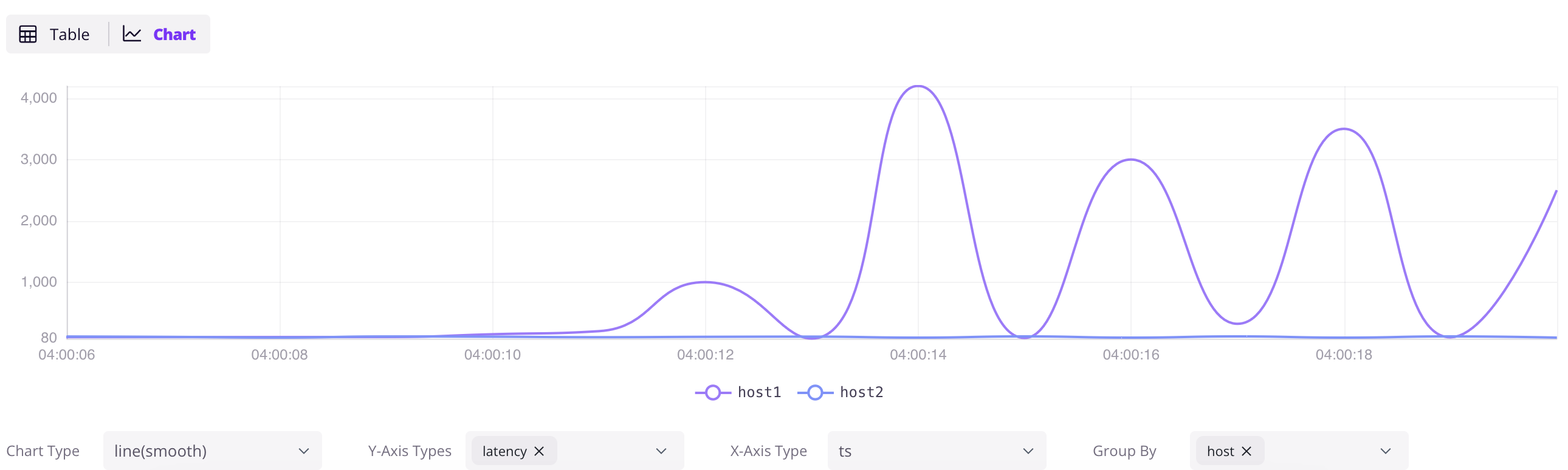
Access the Dashboard at `http://localhost:4000/dashboard`. Click the `+` button to add a query, write SQL, and click `Run All`. Click the `Chart` button in the result panel to visualize the data.
```sql
SELECT * FROM grpc_latencies;
```
### Ingest data by InfluxDB Line Protocol
Click the `Ingest` icon in the Dashboard to write data in [InfluxDB Line Protocol](/user-guide/ingest-data/for-iot/influxdb-line-protocol.md) format. For example:
```txt
grpc_metrics,host=host1,method_name=GetUser latency=100,code=0 1720728021000000000
grpc_metrics,host=host2,method_name=GetUser latency=110,code=1 1720728021000000000
```
Click `Write` to ingest the data. The `grpc_metrics` table is created automatically if it doesn't exist — this is GreptimeDB's [schemaless](/user-guide/ingest-data/overview.md#automatic-schema-generation) capability in action.
## Next steps
**Connect your existing stack:**
- [Prometheus Remote Write](/user-guide/ingest-data/for-observability/prometheus.md) — point your Prometheus at GreptimeDB
- [OpenTelemetry](/user-guide/ingest-data/for-observability/opentelemetry.md) — configure OTel Collector to send metrics, logs, and traces
- [Jaeger](/user-guide/query-data/jaeger.md) — use GreptimeDB as Jaeger's storage backend
- [Loki](/user-guide/ingest-data/for-observability/loki.md) — send logs using Loki protocol
- [Elasticsearch](/user-guide/ingest-data/for-observability/elasticsearch/) — send logs, traces and events using Elasticsearch `_bulk` API
- Find [all ingestion methods](/user-guide/ingest-data/overview/#recommended-data-ingestion-methods).
**Visualize and monitor:**
- [Grafana integration](/user-guide/integrations/grafana.md) — connect Grafana with SQL or PromQL datasource
- [Official Dashboard](/getting-started/installation/greptimedb-dashboard.md) — the embedded dashboard at `http://localhost:4000/dashboard`
**Go deeper:**
- [Why GreptimeDB](/user-guide/concepts/why-greptimedb.md) — architecture, cost comparison, and how GreptimeDB compares
- [Observability 2.0](/user-guide/concepts/observability-2.md) — wide events and the unified data model
- [Demo scene](https://github.com/GreptimeTeam/demo-scene/) — more hands-on examples
- [User Guide](/user-guide/overview.md) — complete reference
---
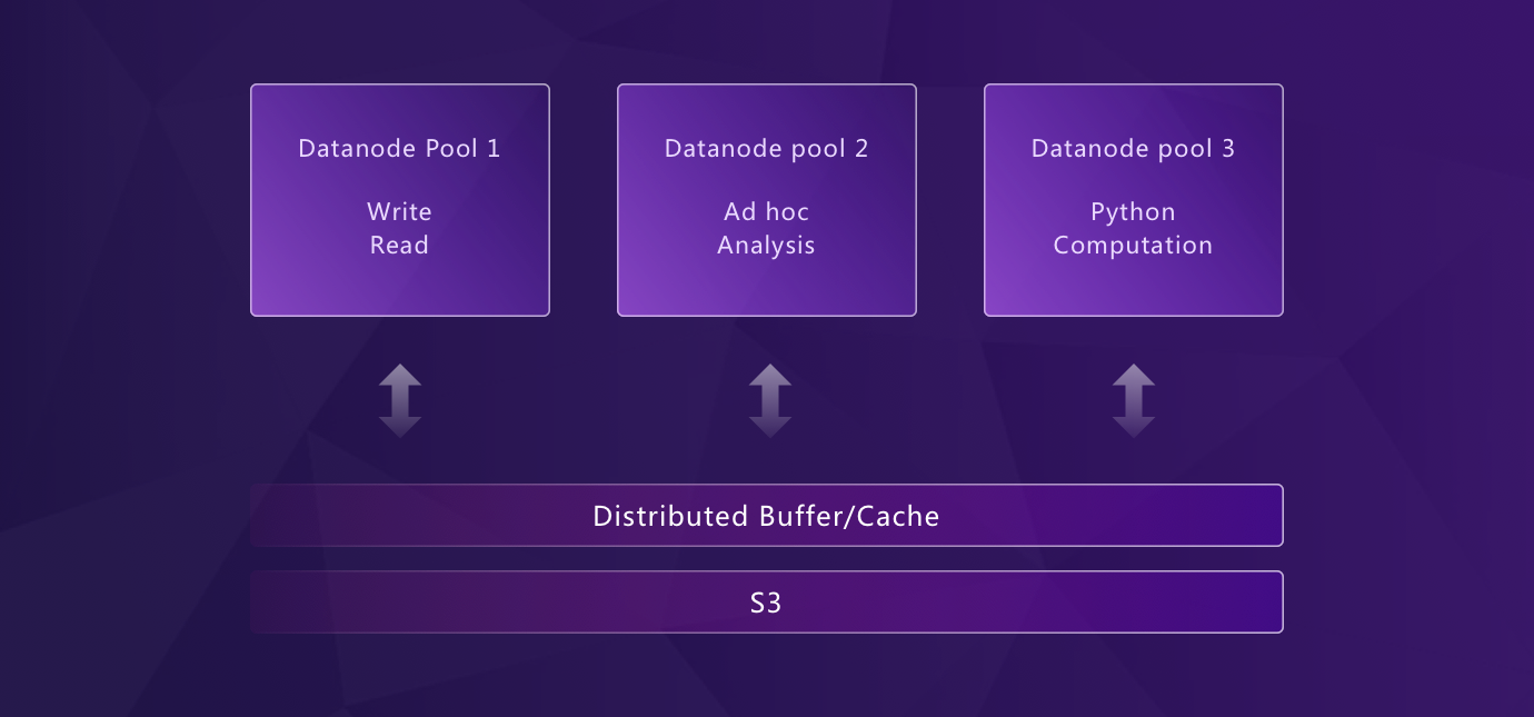
## Architecture
GreptimeDB uses a compute-storage separation architecture where durable data persists in object storage and compute nodes scale independently.
This model supports elastic scaling and lower operational cost compared to architectures that rely on local disks as primary storage.
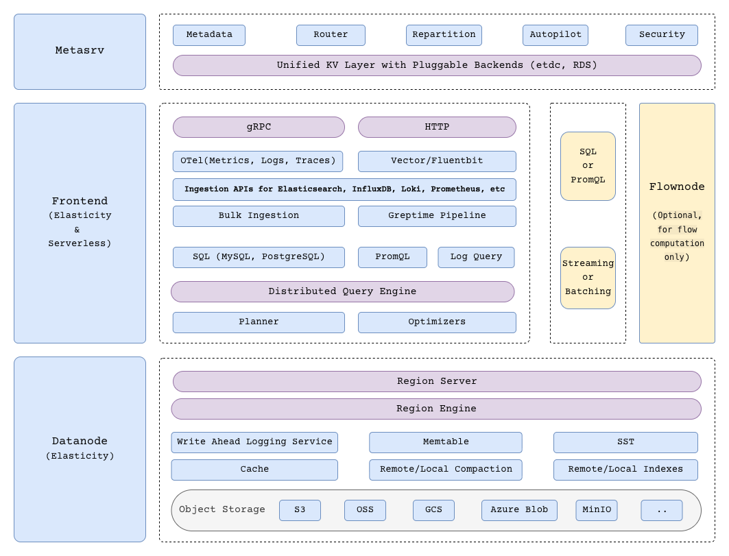
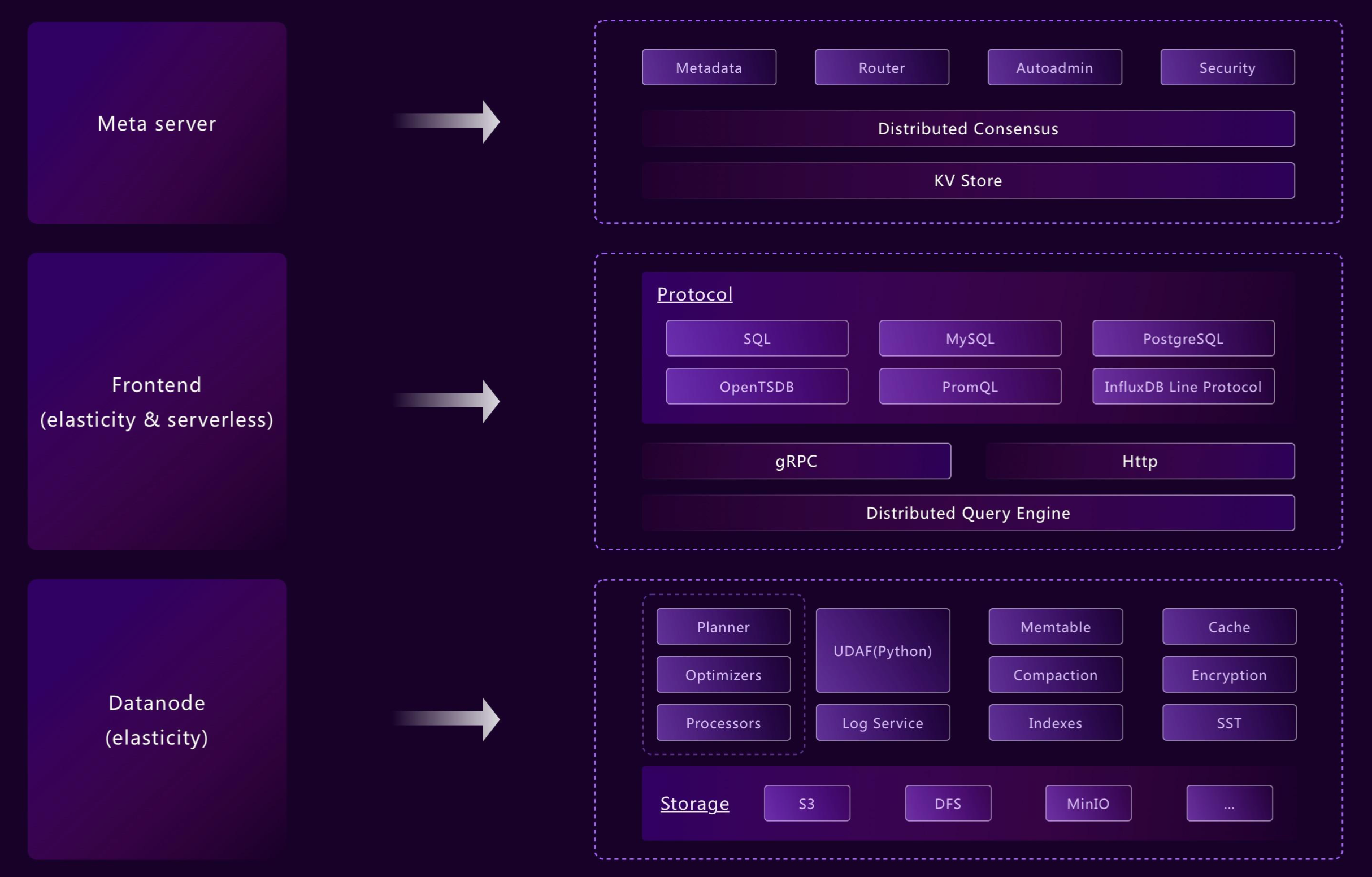
## High-level Architecture
## Components
GreptimeDB has three core components in distributed mode, and one optional component for flow computation:
- [**Metasrv**](/contributor-guide/metasrv/overview.md): Metadata and routing control plane. It manages catalogs/schemas/tables/regions, coordinates scheduling, and serves routing data to other nodes.
- [**Frontend**](/contributor-guide/frontend/overview.md): Stateless access layer. It accepts client protocols, authenticates requests, plans/distributes queries, and routes writes/reads using metadata from Metasrv.
- [**Datanode**](/contributor-guide/datanode/overview.md): Storage and execution layer. It stores table regions, handles reads/writes, persists WAL, and flushes data files to object storage.
- [**Flownode (optional)**](/contributor-guide/flownode/overview.md): Streaming/continuous computation runtime for [Flow Computation](/user-guide/flow-computation/overview.md). It is used when flow workloads run as a separate service in distributed deployments.
In standalone mode, you run one GreptimeDB process instead of managing these services separately.
## How it works
### Write path
1. A client sends write requests to Frontend via supported protocols.
2. Frontend resolves table and region routes from Metasrv metadata (with cache refresh when needed).
3. Frontend splits and forwards requests to target Datanodes.
4. Datanode writes data to memory and [WAL](/user-guide/deployments-administration/wal/overview.md), then eventually flushes immutable data files to [object storage](./storage-location.md).
### Query path
1. A client sends SQL, PromQL, log, or trace queries to Frontend.
2. Frontend creates a distributed plan and dispatches sub-queries to relevant Datanodes.
3. Datanodes execute sub-queries on regions and return partial results.
4. Frontend merges the results and returns the final response.
### Flow path (optional)
When flow computation is enabled, Flownode runs continuous tasks that read source table changes and write computed results to sink tables.
For details, see [Flow Computation](/user-guide/flow-computation/overview.md).
For implementation details, see [Contributor Guide](/contributor-guide/overview.md).
---
## Data Model
## Model
GreptimeDB uses the [time-series](https://en.wikipedia.org/wiki/Time_series) table to guide the organization, compression, and expiration management of data.
The data model is mainly based on the table model in relational databases while considering the characteristics of metrics, logs, and traces data.
All data in GreptimeDB is organized into tables with names. Each data item in a table consists of three semantic types of columns: `Tag`, `Timestamp`, and `Field`.
- Table names are often the same as the indicator names, log source names, or metric names.
- `Tag` columns uniquely identify the time-series.
Rows with the same `Tag` values belong to the same time-series.
Some TSDBs may also call them labels.
- `Timestamp` is the root of a metrics, logs, and traces database.
It represents the date and time when the data was generated.
A table can only have one column with the `Timestamp` semantic type, which is also called the `time index`.
- The other columns are `Field` columns.
Fields contain the data indicators or log contents that are collected.
These fields are generally numerical values or string values,
but may also be other types of data, such as geographic locations or timestamps.
A table clusters rows of the same time-series and sorts rows of the same time-series by `Timestamp`.
The table can also deduplicate rows with the same `Tag` and `Timestamp` values, depending on the requirements of the application.
GreptimeDB stores and processes data by time-series.
Choosing the right schema is crucial for efficient data storage and retrieval; please refer to the [schema design guide](/user-guide/deployments-administration/performance-tuning/design-table.md) for more details.
### Metrics
Suppose we have a table called `system_metrics` that monitors the resource usage of machines in data centers:
```sql
CREATE TABLE IF NOT EXISTS system_metrics (
host STRING,
idc STRING,
cpu_util DOUBLE,
memory_util DOUBLE,
disk_util DOUBLE,
ts TIMESTAMP DEFAULT CURRENT_TIMESTAMP,
PRIMARY KEY(host, idc),
TIME INDEX(ts)
);
```
The data model for this table is as follows:

This is very similar to the table model everyone is familiar with. The difference lies in the `TIME INDEX` constraint, which is used to specify the `ts` column as the time index column of this table.
- The table name here is `system_metrics`.
- The `PRIMARY KEY` constraint specifies the `Tag` columns of the table.
The `host` column represents the hostname of the collected standalone machine.
The `idc` column shows the data center where the machine is located.
- The `Timestamp` column `ts` represents the time when the data is collected.
- The `cpu_util`, `memory_util`, `disk_util`, and `load` columns in the `Field` columns represent
the CPU utilization, memory utilization, disk utilization, and load of the machine, respectively.
These columns contain the actual data.
- The table sorts and deduplicates rows by `host`, `idc`, `ts`. So `select count(*) from system_metrics` will scan all rows.
To learn how GreptimeDB maps Prometheus metrics to this model, see [the documentation](/user-guide/ingest-data/for-observability/prometheus/#data-model).
### Logs
Another example is creating a table for logs like web server access logs:
```sql
CREATE TABLE access_logs (
access_time TIMESTAMP TIME INDEX,
remote_addr STRING,
http_status STRING,
http_method STRING,
http_refer STRING,
user_agent STRING,
request STRING,
) with ('append_mode'='true');
```
- The time index column is `access_time`.
- There are no tags.
- `http_status`, `http_method`, `remote_addr`, `http_refer`, `user_agent` and `request` are fields.
- The table sorts rows by `access_time`.
- The table is an [append-only table](/reference/sql/create.md#create-an-append-only-table) for storing logs that do not support deletion or deduplication.
- Querying an append-only table is usually faster. For example, `select count(*) from access_logs` can use the statistics for result without considering deduplication.
To learn how to indicate `Tag`, `Timestamp`, and `Field` columns, please refer to [table management](/user-guide/deployments-administration/manage-data/basic-table-operations.md#create-a-table) and [CREATE statement](/reference/sql/create.md).
### Traces
GreptimeDB supports writing OpenTelemetry traces data directly via the OTLP/HTTP protocol, refer to the [OTLP traces data model](/user-guide/ingest-data/for-observability/opentelemetry.md#data-model-2) for detail.
## Design Considerations
GreptimeDB is designed on top of the table model for the following reasons:
- The table model has a broad group of users and it's easy to learn; we have simply introduced the concept of time index to metrics, logs, and traces.
- Schema is metadata that describes data characteristics, and it's more convenient for users to manage and maintain.
- Schema brings enormous benefits for optimizing storage and computing with its information like types, lengths, etc., on which we can conduct targeted optimizations.
- When we have the table model, it's natural for us to introduce SQL and use it to process association analysis and aggregation queries between various tables, reducing the learning and usage costs for users.
- GreptimeDB uses a multi-value model where a single row can contain multiple field columns, reducing transfer traffic and simplifying queries compared to single-value models that require splitting data into multiple records. Read the [blog](https://greptime.com/blogs/2024-05-09-prometheus) for detailed benefits.
- In the Observability 2.0 paradigm, metrics, logs, and traces are seen as different projections of the same underlying "wide events." GreptimeDB's unified table model naturally supports this view — all signal types share the same Tag + Timestamp + Field schema, enabling cross-signal correlation in a single SQL query. Read more in [Observability 2.0](./observability-2.md).
GreptimeDB uses SQL to manage table schema. Please refer to [table management](/user-guide/deployments-administration/manage-data/basic-table-operations.md) for more information.
However, our definition of schema is not mandatory and leans towards a **schemaless** approach, similar to MongoDB.
For more details, see [Automatic Schema Generation](/user-guide/ingest-data/overview.md#automatic-schema-generation).
---
## Common Questions
## How does GreptimeDB handle metrics, logs, and traces?
GreptimeDB treats all observability data — metrics, logs, and traces — as timestamped events with context, stored in a unified columnar engine. You can query all three signal types with SQL, use PromQL for metrics, and run continuous aggregations with Flow.
Please read the [log user guide](/user-guide/logs/overview.md) and [traces user guide](/user-guide/traces/overview.md).
## Does GreptimeDB support updates?
Partially supported. See [update data](/user-guide/manage-data/overview.md#update-data) for more information.
## Does GreptimeDB support deletion?
Yes, it does. Please refer to the [delete data](/user-guide/manage-data/overview.md#delete-data) for more information.
## Can I set TTL or retention policy for different tables or measurements?
Of course. Please refer to the document [on managing data retention with TTL policies](/user-guide/manage-data/overview.md#manage-data-retention-with-ttl-policies).
## What are the compression rates of GreptimeDB?
The answer is it depends.
GreptimeDB uses the columnar storage layout, and compresses data by best-in-class algorithms.
And it will select the most suitable compression algorithm based on the column data's statistics and distribution.
GreptimeDB will provide rollups that can compress data more compactly but lose accuracy.
Therefore, the data compression rate of GreptimeDB may be between 2 and several hundred times, depending on the characteristics of your data and whether you can accept accuracy loss.
## How does GreptimeDB address the high cardinality issue?
GreptimeDB resolves high cardinality challenges through a multi-layered approach:
**At the architecture level:**
- **Sharding**: Data and indexes are distributed across region servers, preventing any single node from becoming a bottleneck. Read more about GreptimeDB's [architecture](./architecture.md).
**At the storage level:**
- **Flat format for extreme cardinality**: For workloads with millions of unique series (e.g., request IDs, trace IDs, user tokens as tags), GreptimeDB 1.0+ offers a redesigned storage layout. Traditional time-series databases allocate separate buffers per series, causing memory bloat and degraded performance at scale. Flat format introduces BulkMemtable and multi-series merge paths that eliminate per-series overhead, delivering **4x better write throughput and up to 10x faster queries** in high-cardinality scenarios. Learn more in [Scaling Time Series to Millions of Cardinalities](https://greptime.com/blogs/2025-12-22-flat-format).
**At the indexing level:**
- **Flexible Indexing**: GreptimeDB supports on-demand manual index creation. You can create various index types (inverted, full-text, skipping) for both tag and field columns as needed, rather than automatically indexing every column. This allows you to optimize query performance while minimizing index overhead. Learn more in the [index documentation](/user-guide/manage-data/data-index.md).
**At the query level:**
- **MPP (Massively Parallel Processing)**: The query engine uses vectorized execution and distributed parallel processing to handle high-cardinality queries efficiently across the cluster.
**The result:** GreptimeDB does not hit the same cardinality ceiling as Prometheus, where high-cardinality labels can cause memory exhaustion and query timeouts. Systems can handle millions of series without architectural rewrites.
## Does GreptimeDB support continuous aggregate or downsampling?
Since 0.8, GreptimeDB added a new function called `Flow`, which is used for continuous aggregation. Please read the [user guide](/user-guide/flow-computation/overview.md).
## Can I store data in object storage in the cloud?
Yes, GreptimeDB's data access layer is based on [OpenDAL](https://github.com/apache/incubator-opendal), which supports most kinds of object storage services.
The data can be stored in cost-effective cloud storage services such as AWS S3 or Azure Blob Storage, please refer to storage configuration guide [here](/user-guide/deployments-administration/configuration.md#storage-options).
## How is GreptimeDB's performance compared to other solutions?
[GreptimeDB achieves 1 billion cold run #1 in JSONBench!](https://greptime.com/blogs/2025-03-18-jsonbench-greptimedb-performance)
Please read the performance benchmark reports:
* [GreptimeDB vs. InfluxDB](https://greptime.com/blogs/2024-08-07-performance-benchmark)
* [GreptimeDB vs. TimescaleDB](https://greptime.com/blogs/2025-12-09-greptimedb-vs-timescaledb-benchmark)
* [GreptimeDB vs. Grafana Mimir](https://greptime.com/blogs/2024-08-02-datanode-benchmark)
* [GreptimeDB vs. ClickHouse vs. Elasticsearch](https://greptime.com/blogs/2025-03-10-log-benchmark-greptimedb)
* [GreptimeDB vs. SQLite](https://greptime.com/blogs/2024-08-30-sqlite)
## Does GreptimeDB have disaster recovery solutions?
Yes. Please refer to [disaster recovery](/user-guide/deployments-administration/disaster-recovery/overview.md).
## Does GreptimeDB have geospatial index?
Yes. We offer [built-in functions](/reference/sql/functions/geo.md) for Geohash, H3 and S2 index.
## Any JSON support?
See [JSON functions](/reference/sql/functions/overview.md#json-functions).
## More Questions?
For more comprehensive answers to frequently asked questions about GreptimeDB, including deployment options, migration guides, performance comparisons, and best practices, please visit our [FAQ page](/faq-and-others/faq.md).
---
## Key Concepts
To understand how GreptimeDB manages and serves its data, you need to know about
these building blocks of GreptimeDB.
## Database
Similar to *database* in relational databases, a database is the minimal unit of
data container, within which data can be managed and computed. Users can use the database to achieve data isolation, creating a tenant-like effect.
## Time-Series Table
GreptimeDB designed time-series table to be the basic unit of data storage.
It is similar to a table in a traditional relational database, but requires a timestamp column(We call it **time index**).
The table holds a set of data that shares a common schema, it's a collection of rows and columns:
* Column: a vertical set of values in a table, GreptimeDB distinguishes columns into time index, tag and field.
* Row: a horizontal set of values in a table.
It can be created using SQL `CREATE TABLE`, or inferred from the input data structure using the auto-schema feature.
In a distributed deployment, a table can be split into multiple partitions that sit on different datanodes.
For more information about the data model of the time-series table, please refer to [Data Model](./data-model.md).
## Table Engine
Table engines (also called storage engines) determine how data is stored, managed, and processed within the database. Each engine offers different features, performance characteristics, and trade-offs. GreptimeDB supports `mito` and `metric` engines etc., see [Table Engines](/reference/about-greptimedb-engines.md) for more information.
## Table Region
Each partition of distributed table is called a region. A region may contain a
sequence of continuous data, depending on the partition algorithm. Region
information is managed by Metasrv. It's completely transparent to users who send
write requests or queries.
## Data Types
Data in GreptimeDB is strongly typed. Auto-schema feature provides some
flexibility when creating a table. Once the table is created, data of the same
column must share common data type.
Find all the supported data types in [Data Types](/reference/sql/data-types.md).
## Index
The `index` is a performance-tuning method that allows faster retrieval of records. GreptimeDB provides various kinds of [indexes](/user-guide/manage-data/data-index.md) to accelerate queries.
## View
The `view` is a virtual table that is derived from the result set of a SQL query. It contains rows and columns just like a real table, but it doesn’t store any data itself.
The data displayed in a view is retrieved dynamically from the underlying tables each time the view is queried.
## Flow
A `flow` in GreptimeDB refers to a [continuous aggregation](/user-guide/flow-computation/overview.md) process that continuously updates and materializes aggregated data based on incoming data.
---
## Observability 2.0
Observability 2.0 represents an evolution from the foundational "three pillars" (metrics, logs, and traces) toward a unified data foundation based on high-cardinality, wide-event datasets. Instead of maintaining separate systems for each signal type, this approach emphasizes a single source of truth that enables retroactive analysis rather than pre-aggregation.
Despite its contested naming, the core concept is clear: breaking down the silos between metrics, logs, and traces to provide a more comprehensive view of modern distributed systems.
## The Limits of Three Pillars
For years, observability has relied on the three pillars of metrics, logs, and traces. While these pillars spawned countless successful tools (including [OpenTelemetry](/user-guide/ingest-data/for-observability/opentelemetry.md)), their limitations become evident as systems grow in complexity:
1. **Data silos**: Metrics, logs, and traces are stored separately, leading to uncorrelated datasets. Correlating a spike in error metrics with log patterns requires manual context-switching between systems.
2. **Granularity vs. cost**: Traditional metrics sacrifice detail through pre-aggregation. But retaining full granularity creates millions of time-series with redundant metadata across systems, driving costs up instead of down.
3. **Unstructured logs**: While logs inherently contain structured data, extracting meaning requires intensive parsing, indexing, and computational effort.
These limitations become even more pronounced in modern scenarios like AI agents and microservices, where high-dimensional, semi-structured data is the norm rather than the exception.
## Wide Events: A Unified Data Model
Observability 2.0 addresses these issues by adopting **wide events** as its foundational data structure. A wide event is a context-rich, high-dimensional, and high-cardinality record that captures complete application state in a single event.
### What is a Wide Event?
Instead of precomputing metrics or structuring logs upfront, wide events preserve raw, high-fidelity event data as the single source of truth. For example, a single wide event for a POST request might include:
- User information and subscription data
- Database queries with parameters
- Cache operations
- HTTP headers
- Total: 2KB+ of contextual data in one record
```json
{
"method": "POST",
"path": "/articles",
"service": "articles",
"outcome": "ok",
"status_code": 201,
"duration": 268,
"user": {
"id": "fdc4ddd4-8b30-4ee9-83aa-abd2e59e9603",
"subscription": { "plan": "free", "trial": true }
},
"db": {
"query": "INSERT INTO articles (...)",
"parameters": { "$1": "f8d4d21c-..." }
},
"cache": { "operation": "write", "key": "..." },
"headers": { "user-agent": "...", "cf-connecting-ip": "..." }
}
```
### Metrics, Logs, and Traces as Projections
Wide events fundamentally change how we think about observability data. Metrics, logs, and traces are not separate data types—they are different projections of the same underlying events:
- **Metrics**: `SELECT COUNT(*) GROUP BY status, date_bin(INTERVAL '1' minute, timestamp)` — aggregated projection
- **Logs**: `SELECT message, timestamp WHERE message @@ 'error'` — text projection
- **Traces**: `SELECT span_id, duration WHERE trace_id = '...'` — relational projection
This allows teams to perform exploratory analysis retroactively, deriving any metric, log query, or trace view from the original dataset—without pre-aggregation or code changes.
## AI and the Need for Fine-Grained Observability
AI agents introduce a new level of observability complexity due to their non-deterministic behavior. Unlike traditional applications with predictable code paths, agents make dynamic decisions—choosing tools, reasoning through multi-step plans, and adapting responses based on context. Debugging "why did the agent do X?" requires preserving complete execution state: the full prompt, reasoning chain, tool calls with parameters, memory state, and quality scores—all in a single queryable record.
This is where wide events become essential. Traditional three-pillar approaches fail here: stuffing prompts into logs loses structure and makes analysis impossible, forcing tool calls into traces is too rigid for dynamic behavior, and pre-aggregating token metrics loses the critical context needed for debugging. AI agents produce high-cardinality (millions of unique sessions), high-dimensional (dozens of fields per execution), context-rich events—exactly what wide events are designed to handle. This isn't "observability for the AI age" as a marketing slogan; it's a direct technical consequence: non-deterministic systems require fine-grained, structured, retroactive analysis that only wide events can provide.
## Why GreptimeDB is Built for This
GreptimeDB's [architecture](/user-guide/concepts/architecture.md) naturally aligns with the Observability 2.0 paradigm. Its columnar engine efficiently compresses wide events (achieving 50% storage reduction compared to Loki and ~90% compared to Elasticsearch in production), and [native object storage](/user-guide/concepts/storage-location.md) (S3, Azure Blob, GCS) keeps costs low as wide event volumes grow. Below are the capabilities that matter most for wide events.
### Unified Tag + Timestamp + Field Model
All observability data—metrics, logs, traces—share the same [schema model](/user-guide/concepts/data-model.md) in GreptimeDB:
- **Tags**: Entity identifiers (pod_name, service, region, trace_id, session_id)
- **Timestamp**: Temporal tracking
- **Fields**: Multi-dimensional values (message, duration, status_code, prompts, responses)
This unified model enables cross-signal correlation in a single SQL query.
### SQL + PromQL for Cross-Signal Correlation
Use one [SQL query](/user-guide/query-data/sql.md) to correlate metrics spikes, log patterns, and trace latency:
```sql
SELECT
date_bin(INTERVAL '1' minute, timestamp) AS minute,
COUNT(CASE WHEN status >= 500 THEN 1 END) AS errors,
AVG(duration) AS avg_latency
FROM access_logs
WHERE timestamp >= NOW() - INTERVAL '1' hour
AND message @@ 'timeout'
GROUP BY date_bin(INTERVAL '1' minute, timestamp);
```
No context-switching between systems—all signals in one database. GreptimeDB also supports [PromQL](/user-guide/query-data/promql.md) for metrics queries, maintaining compatibility with existing dashboards.
### Flow Engine for Real-Time Derivation
GreptimeDB's [Flow Engine](/user-guide/flow-computation/overview.md) derives metrics from raw events in real-time without preprocessing pipelines:
```sql
CREATE FLOW http_status_count
SINK TO status_metrics
AS
SELECT
status,
COUNT(*) AS count,
date_bin('1 minute'::INTERVAL, timestamp) AS time_window
FROM access_logs
GROUP BY status, time_window;
```
Metrics are computed continuously from raw wide events, enabling both pre-aggregated dashboards and ad-hoc exploratory queries on the same dataset.
## Wide Events in Production
Wide events are proven in production at scale:
- **Poizon (得物)**: One of the early production deployments of Wide Events. Flow Engine with multi-level continuous aggregation reduced P99 latency from seconds to milliseconds. [Read more →](https://greptime.com/blogs/2025-05-06-poizon-observability-greptimedb-monitoring-use-case)
- **OceanBase Cloud**: One year after migrating from Loki, running 80+ GreptimeDB clusters with 300TB of multi-cloud logs and SQL audit data, with overall log storage cost down by more than 60%. [Read more →](https://greptime.com/blogs/2025-07-22-user-case-obcloud-log-management-greptimedb)
- **Trace Storage**: Replaced [Elasticsearch](/user-guide/protocols/elasticsearch.md) as [Jaeger](/user-guide/query-data/jaeger.md) backend. 45x storage cost reduction, 3x faster cold queries, enabled full-volume tracing at 400B rows/day. [Read more →](https://greptime.com/blogs/2025-04-24-elasticsearch-greptimedb-comparison-performance)
## Getting Started
Transitioning to Observability 2.0 doesn't require ripping out your entire stack. Start from any pillar—[logs](/user-guide/logs/overview.md), [metrics](/user-guide/ingest-data/for-observability/prometheus.md), or [traces](/user-guide/traces/overview.md)—and extend naturally. GreptimeDB supports [PromQL](/user-guide/query-data/promql.md), [Jaeger](/user-guide/query-data/jaeger.md), [OpenTelemetry](/user-guide/ingest-data/for-observability/opentelemetry.md), and [Grafana](/user-guide/integrations/grafana.md) out of the box, so existing dashboards and alerts keep working. See [Why GreptimeDB](./why-greptimedb.md) for detailed migration paths.
## Further Reading
- [Observability 2.0 and the Database for It](https://greptime.com/blogs/2025-04-25-greptimedb-observability2-new-database) — Full vision and technical deep dive
- [Unified Storage for Observability - GreptimeDB's Approach](https://greptime.com/blogs/2024-12-24-observability) — GreptimeDB's unified model philosophy
- [Agent Observability: Can the Old Playbook Handle the New Game?](https://greptime.com/blogs/2025-12-11-agent-observability) — Why AI agents need wide events
- [Scaling Observability at Poizon - Building a Cost-Effective and Real-Time Monitoring Architecture with GreptimeDB](https://greptime.com/blogs/2025-05-06-poizon-observability-greptimedb-monitoring-use-case) — First production-grade validation
- [Beyond Loki! GreptimeDB Log Scenario Performance Report Released](https://greptime.com/blogs/2025-08-07-beyond-loki-greptimedb-log-scenario-performance-report) — Logs pillar migration
- [Beyond ELK: Lightweight and Scalable Cloud-Native Log Monitoring](https://greptime.com/blogs/2025-04-24-elasticsearch-greptimedb-comparison-performance) — Traces pillar migration
---
## GreptimeDB Concepts Overview
# Concepts
GreptimeDB is an observability database that unifies metrics, logs, and traces in a single engine. This section covers the core concepts you need to understand how GreptimeDB works and why it's designed this way.
**Start here:**
- [Why GreptimeDB](./why-greptimedb.md) — The problem with three-pillar observability stacks, and how GreptimeDB solves it
- [Data Model](./data-model.md) — How metrics, logs, and traces are represented as timestamped events with tags and fields
- [Architecture](./architecture.md) — Compute-storage separation, stateless frontends, and how GreptimeDB scales
**Deep dives:**
- [Observability 2.0](./observability-2.md) — Wide events, unified data model, and the evolution beyond three pillars
- [Storage Location](./storage-location.md) — Object storage, local disk, and multi-engine storage options
- [Key Concepts](./key-concepts.md) — Tables, regions, time index, data types, views, and flows
- [Common Questions](./features-that-you-concern.md) — FAQ on updates, deletions, TTL, compression, high cardinality, and more
## Further Reading
- [Observability 2.0 and the Database for It](https://greptime.com/blogs/2025-04-25-greptimedb-observability2-new-database) — Our vision for the next generation of observability
- [Unifying Logs and Metrics](https://greptime.com/blogs/2024-06-25-logs-and-metrics)
- [GreptimeDB Storage Engine Design](https://greptime.com/blogs/2022-12-21-storage-engine-design)
---
## Storage Location
GreptimeDB supports storing data in local file system, AWS S3 and compatible services (including minio, digitalocean space, Tencent Cloud Object Storage(COS), Baidu Object Storage(BOS) and so on), Azure Blob Storage and Aliyun OSS.
## Local File Structure
The storage file structure of GreptimeDB includes of the following:
```cmd
├── metadata
├── raftlog
├── rewrite
└── LOCK
├── data
│ ├── greptime
│ └── public
├── cache
├── logs
├── index_intermediate
│ └── staging
└── wal
├── raftlog
├── rewrite
└── LOCK
```
- `metadata`: The internal metadata directory that keeps catalog, database and table info, procedure states, etc. In cluster mode, this directory does not exist, because all those states including region route info are saved in `Metasrv`.
- `data`: The files in data directory store time series data and index files of GreptimeDB. To customize this path, please refer to [Storage option](/user-guide/deployments-administration/configuration.md#storage-options). The directory is organized in a two-level structure of catalog and schema.
- `cache`: The directory for internal caching, such as object storage cache, etc.
- `logs`: The log files contains all the logs of operations in GreptimeDB.
- `wal`: The wal directory contains the write-ahead log files.
- `index_intermediate`: the temporary intermediate data while indexing.
## Cloud storage
The `data` directory in the file structure can be stored in cloud storage. Please refer to [Storage option](/user-guide/deployments-administration/configuration.md#storage-options) for more details.
Please note that only storing the data directory in object storage is not sufficient to ensure data reliability and disaster recovery. The `wal` and `metadata` also need to be considered for disaster recovery. Please refer to the [disaster recovery documentation](/user-guide/deployments-administration/disaster-recovery/overview.md).
## Multiple storage engines
Another powerful feature of GreptimeDB is that you can choose the storage engine for each table. For example, you can store some tables on the local disk, and some tables in Amazon S3 or Google Cloud Storage, see [create table](/reference/sql/create.md#create-table).
---
## Why GreptimeDB
## The Problem: Three Systems for Three Signals
Most observability stacks today look like this: [Prometheus](/user-guide/ingest-data/for-observability/prometheus.md) (or Thanos/Mimir) for metrics, [Grafana Loki](/user-guide/ingest-data/for-observability/loki.md) (or ELK) for logs, and [Elasticsearch](/user-guide/protocols/elasticsearch.md) (or Tempo) for traces. Each system has its own query language, storage backend, scaling model, and operational overhead.
This "three pillars" architecture made sense when these were separate concerns. But in practice, it means:
- **3x operational complexity** — three systems to deploy, monitor, upgrade, and debug
- **Data silos** — correlating a spike in error logs with a metrics anomaly requires manual context-switching between systems
- **Cost escalation** — each system stores redundant metadata, and scaling each independently leads to over-provisioning
GreptimeDB takes a different approach: one database engine for all three signal types, built on object storage with compute-storage separation.
## Unified Processing for Observability Data
GreptimeDB unifies the processing of metrics, logs, and traces through:
- A consistent [data model](./data-model.md) that treats all observability data as timestamped wide events with context
- Native support for both [SQL](/user-guide/query-data/sql.md) and [PromQL](/user-guide/query-data/promql.md) queries
- Built-in stream processing capabilities ([Flow](/user-guide/flow-computation/overview.md)) for real-time aggregation and analytics
- Seamless correlation analysis across different types of observability data (read the [SQL example](/getting-started/quick-start.md#correlate-metrics-logs-and-traces) for detailed info)
It replaces complex legacy data stacks with a high-performance single solution.
This means you can replace the [Prometheus](/user-guide/ingest-data/for-observability/prometheus.md) + [Loki](/user-guide/ingest-data/for-observability/loki.md) + [Elasticsearch](/user-guide/protocols/elasticsearch.md) stack with a single database, and use SQL to correlate metrics spikes with log patterns and trace latency — in one query, without context-switching between systems.
## Cost-Effective with Object Storage
GreptimeDB leverages [cloud object storage](/user-guide/concepts/storage-location.md) (like AWS S3 and Azure Blob Storage etc.) as its storage layer, dramatically reducing costs compared to traditional storage solutions. Its optimized columnar storage and advanced compression algorithms achieve up to 50x cost efficiency. Scale flexibly across cloud storage systems (e.g., S3, Azure Blob Storage) for simplified management, dramatic cost efficiency, and **no vendor lock-in**.
In production deployments, teams have achieved:
- **Logs**: 60%+ storage cost reduction in production at OceanBase Cloud (migrated from [Loki](/user-guide/ingest-data/for-observability/loki.md) — 80+ GreptimeDB clusters, 300TB of multi-cloud logs and SQL audit data)
- **Traces**: 45x storage cost reduction, 3x faster queries (replaced [Elasticsearch](/user-guide/protocols/elasticsearch.md) as [Jaeger](/user-guide/query-data/jaeger.md) backend — one-week migration)
- **Metrics**: Replaced Thanos with native compute-storage separation, significantly reducing operational complexity
## High Performance
As for performance optimization, GreptimeDB utilizes different techniques such as LSM Tree, data sharding, and flexible WAL options (local disk or distributed services like Kafka), to handle large workloads of observability data ingestion.
GreptimeDB is written in pure Rust for superior performance and reliability. The powerful and fast query engine is powered by vectorized execution and distributed parallel processing (thanks to [Apache DataFusion](https://datafusion.apache.org/)), and combined with [indexing capabilities](/user-guide/manage-data/data-index.md) such as inverted index, skipping index, and full-text index. GreptimeDB combines smart indexing and Massively Parallel Processing (MPP) to boost pruning and filtering.
[GreptimeDB achieves 1 billion cold runs #1 in JSONBench!](https://greptime.com/blogs/2025-03-18-jsonbench-greptimedb-performance) Read more [benchmark reports](https://www.greptime.com/blogs/2024-09-09-report-summary).
## Elastic Scaling with Kubernetes
Built from the ground up for [Kubernetes](/user-guide/deployments-administration/deploy-on-kubernetes/overview.md), GreptimeDB features a disaggregated storage and compute [architecture](/user-guide/concepts/architecture.md) that enables true elastic scaling:
- Independent scaling of storage and compute resources
- Unlimited horizontal scalability through Kubernetes
- Resource isolation between different workloads (ingestion, querying, compaction)
- Automatic failover and high availability
Unlike Thanos or Mimir, which require multiple stateful components (ingesters with persistent disks, store-gateways, compactors) to achieve scalability, GreptimeDB's architecture separates compute from storage at the core — data persists in object storage, compute nodes scale independently, with local disk serving as buffer/cache. WAL can be configured flexibly (local or distributed via Kafka). Scaling up means adding nodes; scaling down loses no data.
## Flexible Architecture: From Edge to Cloud
GreptimeDB's modularized [architecture](/user-guide/concepts/architecture.md) allows different components to operate independently or in unison as needed. Its flexible design supports a wide variety of deployment scenarios, from edge devices to cloud environments, while still using consistent APIs for operations. For example:
- Frontend, datanode, and metasrv can be merged into a standalone binary
- Components like WAL or indexing can be enabled or disabled per table
This flexibility ensures that GreptimeDB meets deployment requirements for edge-to-cloud solutions, like the [Edge-Cloud Integrated Solution](https://greptime.com/product/carcloud).
From embedded and standalone deployments to cloud-native clusters, GreptimeDB adapts to various environments easily.
## Easy to Integrate
GreptimeDB supports [PromQL](/user-guide/query-data/promql.md), [Prometheus remote write](/user-guide/ingest-data/for-observability/prometheus.md), [OpenTelemetry](/user-guide/ingest-data/for-observability/opentelemetry.md), [Jaeger](/user-guide/query-data/jaeger.md), [Loki](/user-guide/ingest-data/for-observability/loki.md), [Elasticsearch](/user-guide/protocols/elasticsearch.md), [MySQL](/user-guide/protocols/mysql.md), and [PostgreSQL](/user-guide/protocols/postgresql.md) protocols — migrate from your existing stack without rewriting queries or pipelines. Query with [SQL](/user-guide/query-data/sql.md) or PromQL, visualize with [Grafana](/user-guide/integrations/grafana.md).
The combination of SQL and PromQL means GreptimeDB can replace the classic "Prometheus + data warehouse" combo — use PromQL for real-time monitoring and alerting, SQL for deep analytics, joins, and aggregations, all in one system. GreptimeDB also supports a [multi-value model](/user-guide/concepts/data-model.md), where a single row can contain multiple field columns, reducing transfer traffic and simplifying queries compared to single-value models.
Beyond querying, SQL is also GreptimeDB's management interface — [create tables](/user-guide/deployments-administration/manage-data/basic-table-operations.md), [manage schemas](/reference/sql/alter.md), set [TTL policies](/user-guide/manage-data/overview.md#manage-data-retention-with-ttl-policies), and configure [indexes](/user-guide/manage-data/data-index.md), all through standard SQL. No proprietary config files, no custom APIs, no YAML-driven control planes. This is a key operational difference from systems like Prometheus (configured via YAML + relabeling rules), Loki (LogQL + config files), or Elasticsearch (REST API + JSON mappings). Teams with SQL skills can manage GreptimeDB without learning new tooling.
## How GreptimeDB Compares
The following comparison is based on general architectural characteristics and typical deployment scenarios:
| | GreptimeDB | Prometheus / Thanos / Mimir | Grafana Loki | Elasticsearch |
|---|---|---|---|---|
| Data types | Metrics, logs, traces | Metrics only | Logs only | Logs, traces |
| Query language | SQL + PromQL | PromQL | LogQL | Query DSL |
| Storage | Native object storage (S3, etc.) | Local disk + object storage (Thanos/Mimir), ingester requires persistent disk | Object storage (chunks) | Local disk |
| Scaling | Compute-storage separation, compute nodes scale independently | Federation / Thanos / Mimir — multi-component, ops heavy | Stateless + object storage | Shard-based, ops heavy |
| Cost efficiency | Up to 50x lower storage | High at scale | Moderate | High (inverted index overhead) |
| OpenTelemetry | Native (metrics + logs + traces) | Partial (metrics only) | Partial (logs only) | Via instrumentation |
| Management | Standard SQL (DDL, TTL, indexes) | YAML config + relabeling rules | YAML config + LogQL | REST API + JSON mappings |
For more details, explore:
- [Observability 2.0](./observability-2.md) — Wide events, unified data model, and GreptimeDB's architecture for the next generation of observability
- [Unified Storage for Observability - GreptimeDB's Approach](https://greptime.com/blogs/2024-12-24-observability) — GreptimeDB's approach to unified storage
- [Beyond Loki: Lightweight and Scalable Cloud-Native Log Monitoring](https://greptime.com/blogs/2025-08-07-beyond-loki-greptimedb-log-scenario-performance-report)
---
## Authentication
Authentication occurs when a user attempts to connect to the database. In GreptimeDB, users are authenticated by "user
provider"s. There are various implementations of user providers in GreptimeDB:
- [Static User Provider](./static.md): A simple built-in user provider implementation that finds users from a static
file.
- [LDAP User Provider](/enterprise/deployments-administration/authentication.md): **Enterprise feature.** A user provider implementation that authenticates users against an external LDAP
server.
---
## Static User Provider
GreptimeDB offers a simple built-in mechanism for authentication, allowing users to configure either a fixed account for convenient usage or an account file for multiple user accounts. By passing in a file, GreptimeDB loads all users listed within it.
## Standalone Mode
GreptimeDB reads the user configuration from a file where each line defines a user with their password and optional permission mode.
### Basic Configuration
The basic format uses `=` as a separator between username and password:
```
greptime_user=greptime_pwd
alice=aaa
bob=bbb
```
Users configured this way have full read-write access by default.
### Permission Modes
You can optionally specify permission modes to control user access levels. The format is:
```
username:permission_mode=password
```
Available permission modes:
- `rw` or `readwrite` - Full read and write access (default when not specified)
- `ro` or `readonly` - Read-only access
- `wo` or `writeonly` - Write-only access
Example configuration with mixed permission modes:
```
admin=admin_pwd
alice:readonly=aaa
bob:writeonly=bbb
viewer:ro=viewer_pwd
editor:rw=editor_pwd
```
In this configuration:
- `admin` has full read-write access (default)
- `alice` has read-only access
- `bob` has write-only access
- `viewer` has read-only access
- `editor` has explicitly set read-write access
### Starting the Server
Start the server with the `--user-provider` parameter and set it to `static_user_provider:file:` (replace `` with the path to your user configuration file):
```shell
./greptime standalone start --user-provider=static_user_provider:file:
```
The users and their permissions will be loaded into GreptimeDB's memory. You can create connections to GreptimeDB using these user accounts with their respective access levels enforced.
:::tip Note
When using `static_user_provider:file`, the file’s contents are loaded at startup. Changes or additions to the file have no effect while the database is running.
:::
### Dynamic File Reloading
If you need to update user credentials without restarting the server, you can use the `watch_file_user_provider` instead of `static_user_provider:file`. This provider monitors the credential file for changes and automatically reloads it:
```shell
./greptime standalone start --user-provider=watch_file_user_provider:
```
The watch file provider:
- Uses the same file format as the static file provider
- Automatically detects file modifications and reloads credentials
- Allows adding, removing, or modifying users without server restart
- If the file is temporarily unavailable or invalid, it keeps the last valid configuration
This is particularly useful in production environments where you need to manage user access dynamically.
## Kubernetes Cluster
You can configure the authentication users in the `values.yaml` file.
For more details, please refer to the [Helm Chart Configuration](/user-guide/deployments-administration/deploy-on-kubernetes/common-helm-chart-configurations.md#authentication-configuration).
---
## Capacity Plan
This guide provides general advice on the CPU, memory, and storage requirements for GreptimeDB.
GreptimeDB is designed to be lightweight upon startup,
which allows for the database to be initiated with minimal server resources.
However, when configuring your server capacity for a production environment,
there are several key considerations:
- Data points processed per second
- Query requests per second
- Data volume
- Data retention policy
- Hardware costs
To monitor the various metrics of GreptimeDB, please refer to [Monitoring](/user-guide/deployments-administration/monitoring/overview.md).
## CPU
Generally, applications that handle many concurrent queries, process large amounts of data,
or perform other compute-intensive operations will require more CPU cores.
Here are some recommendations for CPU resource usage,
but the actual number of CPUs you should use depends on your workload.
Consider allocating 30% of your CPU resources for data ingestion,
with the remaining 70% to querying and analytics.
A recommended guideline for resource allocation is to maintain a CPU to memory ratio of 1:4 (for instance, 8 core to 32 GB).
However, if your workload consists primarily of data ingestion with few queries,
a ratio of 1:2 (8 core to 16 GB) can also be acceptable.
## Memory
In general, the more memory you have, the faster your queries will run.
For basic workloads, it's recommended to have at least 8 GB of memory, and 32 GB for more advanced ones.
## Storage
GreptimeDB features an efficient data compaction mechanism that reduces the original data size to about 1/8 to 1/10 of its initial volume.
This allows GreptimeDB to store large amounts of data in a significantly smaller space.
Data can be stored either in a local file system or in cloud storage, such as AWS S3.
FOr more information on storage options,
please refer to the [storage configuration](/user-guide/deployments-administration/configuration.md#storage-options) documentation.
Cloud storage is highly recommended for data storage due to its simplicity in managing storage.
With cloud storage, only about 200GB of local storage space is needed for query-related caches and Write-Ahead Log (WAL).
In order to manage the storage costs effectively,
it is recommended setting a [retention policy](/user-guide/concepts/features-that-you-concern.md#can-i-set-ttl-or-retention-policy-for-different-tables-or-measurements).
## Example
Consider a scenario where your database handles a query rate of about 200 simple queries per second (QPS) and an ingestion rate of approximately 300k data points per second, using cloud storage for data.
Given the high ingestion and query rates,
here's an example of how you might allocate resources:
- CPU: 8 cores
- Memory: 32 GB
- Storage: 200 GB
Such an allocation is designed to optimize performance,
ensuring smooth data ingestion and query processing without system overload.
However, remember these are just guidelines,
and actual requirements may vary based on specific workload characteristics and performance expectations.
---
## GreptimeDB Deployment Configuration
# Configuration
GreptimeDB supports **layered configuration** with the following precedence order (where each item overrides the one below it):
- Greptime command line options
- Configuration file options
- Environment variables
- Default values
You only need to set up the configurations you require.
GreptimeDB will assign default values for any settings not configured.
## How to set up configurations
### Greptime command line options
You can specify several configurations using command line arguments.
For example, to start GreptimeDB in standalone mode with a configured HTTP address:
```shell
greptime standalone start --http-addr 127.0.0.1:4000
```
For all the options supported by the Greptime command line,
refer to the [GreptimeDB Command Line Interface](/reference/command-lines/overview.md).
### Configuration file options
You can specify configurations in a TOML file.
For example, create a configuration file `standalone.example.toml` as shown below:
```toml
[storage]
type = "File"
data_home = "greptimedb_data"
```
Then, specify the configuration file using the command line argument `-c [file_path]`.
```sh
greptime [standalone | frontend | datanode | metasrv] start -c config/standalone.example.toml
```
For example, to start in standalone mode:
```bash
greptime standalone start -c standalone.example.toml
```
#### Example files
Below are example configuration files for each GreptimeDB component,
including all available configurations.
In actual scenarios,
you only need to configure the required options and do not need to configure all options as in the sample file.
- [standalone](https://github.com/GreptimeTeam/greptimedb/blob/v1.0.2/config/standalone.example.toml)
- [frontend](https://github.com/GreptimeTeam/greptimedb/blob/v1.0.2/config/frontend.example.toml)
- [datanode](https://github.com/GreptimeTeam/greptimedb/blob/v1.0.2/config/datanode.example.toml)
- [flownode](https://github.com/GreptimeTeam/greptimedb/blob/v1.0.2/config/flownode.example.toml)
- [metasrv](https://github.com/GreptimeTeam/greptimedb/blob/v1.0.2/config/metasrv.example.toml)
### Helm Configurations
When deploying GreptimeDB on Kubernetes using Helm charts,
you can configure certain settings directly in the Helm `values.yaml` file.
Please refer to the [Helm configuration documentation](/user-guide/deployments-administration/deploy-on-kubernetes/common-helm-chart-configurations.md) for all Helm-supported configurations.
For configurations that are available only in the [options](#options) section of this document,
you can [inject complete TOML configuration files](/user-guide/deployments-administration/deploy-on-kubernetes/common-helm-chart-configurations.md#injecting-configuration-files) into your deployment.
### Environment variable
Every item in the configuration file can be mapped to environment variables.
For example, to set the `data_home` configuration item for the datanode using an environment variable:
```toml
# ...
[storage]
data_home = "/data/greptimedb"
# ...
```
Use the following shell command to set the environment variable in the following format:
```
export GREPTIMEDB_DATANODE__STORAGE__DATA_HOME=/data/greptimedb
```
#### Environment Variable Rules
- Each environment variable should have the component prefix, for example:
- `GREPTIMEDB_FRONTEND`
- `GREPTIMEDB_METASRV`
- `GREPTIMEDB_DATANODE`
- `GREPTIMEDB_STANDALONE`
- Use **double underscore `__`** separators. For example, the data structure `storage.data_home` is transformed to `STORAGE__DATA_HOME`.
The environment variable also accepts lists that are separated by commas `,`, for example:
```
GREPTIMEDB_METASRV__META_CLIENT__METASRV_ADDRS=127.0.0.1:3001,127.0.0.1:3002,127.0.0.1:3003
```
## Options
In this section, we will introduce some main configuration options.
For all options, refer to the [Configuration Reference](https://github.com/GreptimeTeam/greptimedb/blob/v1.0.2/config/config.md) on Github.
### Write memory limiter options
Memory limiter options control the total memory used by concurrent write requests across all protocols (HTTP, gRPC, and Arrow Flight).
These options are valid in `frontend` and `standalone` subcommands.
```toml
# Maximum total memory for all concurrent write request bodies and messages
# Set to 0 to disable the limit (unlimited by default)
max_in_flight_write_bytes = "1GB"
# Policy when write bytes quota is exhausted
# Options: "wait" (default, 10s timeout), "wait()" (e.g., "wait(30s)"), "fail"
write_bytes_exhausted_policy = "wait"
```
| Option | Type | Default | Description |
| ------------------------------- | ------ | ------- | ----------------------------------------------------------------------------------------------------------------------------------------------------------------------------------------------------------------------------------------------------- |
| `max_in_flight_write_bytes` | String | `"0"` | Maximum total memory for all concurrent write request bodies and messages (HTTP, gRPC, Flight). Set to `"0"` to disable the limit (unlimited). Supports units: `B`, `KB`, `MB`, `GB`, etc. Example: `"1GB"` limits total concurrent writes to 1GB. |
| `write_bytes_exhausted_policy` | String | `"wait"`| Policy when write bytes quota is exhausted. Options: `"wait"` (default, waits up to 10 seconds), `"wait()"` (custom timeout, e.g., `"wait(30s)"`), `"fail"` (immediately reject the request). |
### Protocol options
Protocol options are valid in `frontend` and `standalone` subcommands,
specifying protocol server addresses and other protocol-related options.
:::tip NOTE
The HTTP protocol configuration is available for all GreptimeDB components: `frontend`, `datanode`, `flownode`, and `metasrv`.
:::
Below is an example configuration with default values.
You can change the values or disable certain protocols in your configuration file.
For example, to disable OpenTSDB protocol support, set the `enable` parameter to `false`.
Note that HTTP and gRPC protocols cannot be disabled for the database to function correctly.
```toml
[http]
addr = "127.0.0.1:4000"
timeout = "0s"
body_limit = "64MB"
[grpc]
bind_addr = "127.0.0.1:4001"
runtime_size = 8
[mysql]
enable = true
addr = "127.0.0.1:4002"
runtime_size = 2
[mysql.tls]
mode = "disable"
cert_path = ""
key_path = ""
watch = false
[postgres]
enable = true
addr = "127.0.0.1:4003"
runtime_size = 2
[postgres.tls]
mode = "disable"
cert_path = ""
key_path = ""
watch = false
[opentsdb]
enable = true
[influxdb]
enable = true
[prom_store]
enable = true
with_metric_engine = true
```
The following table describes the options in detail:
| Option | Key | Type | Description |
| ---------- | -------------------- | ------- | ------------------------------------------------------------------------------------------------------------------------------------------------------------------------------------------------------------------------------------------------------------------------------------------------------------------------------------------------------------------------------------------ |
| http | | | HTTP server options |
| | addr | String | Server address, "127.0.0.1:4000" by default |
| | timeout | String | HTTP request timeout. Set to 0 to disable timeout (default: "0s"). |
| | body_limit | String | HTTP max body size, "64MB" by default |
| | prom_validation_mode | String | Whether to check if strings are valid UTF-8 strings in Prometheus remote write requests. Available options: `strict`(reject any request with invalid UTF-8 strings), `lossy`(replace invalid characters with [UTF-8 REPLACEMENT CHARACTER U+FFFD, which looks like �](https://www.unicode.org/versions/Unicode16.0.0/core-spec/chapter-23/#G24272)), `unchecked`(do not validate strings). |
| grpc | | | gRPC server options |
| | bind_addr | String | The address to bind the gRPC server, "127.0.0.1:4001" by default |
| | runtime_size | Integer | The number of server worker threads, 8 by default |
| | max_connection_age | String | Maximum lifetime of a gRPC connection that the server keeps it. Refer to ["MAX_CONNECTION_AGE"](https://grpc.io/docs/guides/keepalive/) for details. Defaults to not set. Example: "1h" for 1 hour, "30m" for 30 minutes |
| | flight_compression | String | Compression mode for frontend side Arrow IPC service. Available options: `none`: disable all compression, `transport`: only enable gRPC transport compression (zstd), `arrow_ipc`: only enable Arrow IPC compression (lz4), `all`: enable all compression. Default value is `none`. |
| mysql | | | MySQL server options |
| | enable | Boolean | Whether to enable MySQL protocol, true by default |
| | addr | String | Server address, "127.0.0.1:4002" by default |
| | runtime_size | Integer | The number of server worker threads, 2 by default |
| influxdb | | | InfluxDB Protocol options |
| | enable | Boolean | Whether to enable InfluxDB protocol in HTTP API, true by default |
| opentsdb | | | OpenTSDB Protocol options |
| | enable | Boolean | Whether to enable OpenTSDB protocol in HTTP API, true by default |
| prom_store | | | Prometheus remote storage options |
| | enable | Boolean | Whether to enable Prometheus Remote Write and read in HTTP API, true by default |
| | with_metric_engine | Boolean | Whether to use the metric engine on Prometheus Remote Write, true by default |
| postgres | | | PostgresSQL server options |
| | enable | Boolean | Whether to enable PostgresSQL protocol, true by default |
| | addr | String | Server address, "127.0.0.1:4003" by default |
| | runtime_size | Integer | The number of server worker threads, 2 by default |
For MySQL, Postgres and gRPC interface, TLS can be configured to enable transport
layer security.
| Option | Key | Type | Description |
| ----------------------------------------- | ----------- | ------- | ------------------------------------------------------------- |
| `mysql.tls`, `postgres.tls` or `grpc.tls` | | | TLS configuration for MySQL and Postgres |
| | `mode` | String | TLS mode, options are `disable`, `prefer` and `require` |
| | `cert_path` | String | File path for TLS certificate |
| | `key_path` | String | File path for TLS private key |
| | `watch` | Boolean | Watch file system changes and reload certificate and key file |
### Query options
The `query` options are valid in standalone, datanode and frontend modes, which controls the query engine's behavior.
The following table describes the options in detail:
| Option | Key | Type | Description |
| ----------- | ------- | ---- | ----------------------------------------------------------------------------------- |
| parallelism | Integer | `0` | Parallelism of the query engine. Default to 0, which means the number of CPU cores. |
A sample configuration:
```toml
[query]
parallelism = 0
```
### Storage options
The `storage` options are valid in datanode and standalone mode, which specify the database data directory and other storage-related options.
GreptimeDB supports storing data in local file system, AWS S3 and compatible services (including MinIO, digitalocean space, Tencent Cloud Object Storage(COS), Baidu Object Storage(BOS) and so on), Azure Blob Storage and Aliyun OSS.
| Option | Key | Type | Description |
| ------- | ------------------------- | ------- | -------------------------------------------------------------------------------- |
| storage | | | Storage options |
| | type | String | Storage type, supports "File", "S3" and "Oss" etc. |
| File | | | Local file storage options, valid when type="File" |
| | data_home | String | Database storage root directory, "./greptimedb_data" by default |
| S3 | | | AWS S3 storage options, valid when type="S3" |
| | name | String | The storage provider name, default is `S3` |
| | bucket | String | The S3 bucket name |
| | root | String | The root path in S3 bucket |
| | endpoint | String | The API endpoint of S3 |
| | region | String | The S3 region |
| | access_key_id | String | The S3 access key id |
| | secret_access_key | String | The S3 secret access key |
| | enable_virtual_host_style | Boolean | Send API requests in virtual host style instead of path style. Default is false. |
| Oss | | | Aliyun OSS storage options, valid when type="Oss" |
| | name | String | The storage provider name, default is `Oss` |
| | bucket | String | The OSS bucket name |
| | root | String | The root path in OSS bucket |
| | endpoint | String | The API endpoint of OSS |
| | access_key_id | String | The OSS AccessKey ID |
| | access_key_secret | String | The OSS AccessKey Secret |
| Azblob | | | Azure Blob Storage options, valid when type="Azblob" |
| | name | String | The storage provider name, default is `Azblob` |
| | container | String | The container name |
| | root | String | The root path in container |
| | endpoint | String | The API endpoint of Azure Blob Storage |
| | account_name | String | The account name of Azure Blob Storage |
| | account_key | String | The access key |
| | sas_token | String | The shared access signature |
| Gsc | | | Google Cloud Storage options, valid when type="Gsc" |
| | name | String | The storage provider name, default is `Gsc` |
| | root | String | The root path in Gsc bucket |
| | bucket | String | The Gsc bucket name |
| | scope | String | The Gsc service scope |
| | credential_path | String | The Gsc credentials path |
| | endpoint | String | The API endpoint of Gsc |
A file storage sample configuration:
```toml
[storage]
type = "File"
data_home = "./greptimedb_data/"
```
A S3 storage sample configuration:
```toml
[storage]
type = "S3"
bucket = "test_greptimedb"
root = "/greptimedb"
access_key_id = ""
secret_access_key = ""
```
### Storage http client
`[storage.http_client]` sets the options for the http client that is used to send requests to the storage service.
Only applied for storage types "S3", "Oss", "Azblob" and "Gcs".
| Key | Type | Default | Description |
| ------------------------ | ------- | ------------------ | -------------------------------------------------------------------------------------------------------------------------------------------------- |
| `pool_max_idle_per_host` | Integer | 1024 | The maximum idle connection per host allowed in the pool. |
| `connect_timeout` | String | "30s" (30 seconds) | The timeout for only the connect phase of a http client. |
| `timeout` | String | "30s" (30 seconds) | The total request timeout, applied from when the request starts connecting until the response body has finished. Also considered a total deadline. |
| `pool_idle_timeout` | String | "90s" (90 seconds) | The timeout for idle sockets being kept-alive. |
### Storage engine provider
`[[storage.providers]]` setups the table storage engine providers. Based on these providers, you can create a table with a specified storage, see [create table](/reference/sql/create.md#create-table):
```toml
# Allows using multiple storages
[[storage.providers]]
name = "S3"
type = "S3"
bucket = "test_greptimedb"
root = "/greptimedb"
access_key_id = ""
secret_access_key = ""
[[storage.providers]]
name = "Gcs"
type = "Gcs"
bucket = "test_greptimedb"
root = "/greptimedb"
credential_path = ""
```
All configured providers' names can be used as the `storage` option when creating tables.
For storage from the same provider, if you want to use different S3 buckets as storage engines for different tables, you can set different `name` values and specify the `storage` option when creating the table.
### Object storage cache
When using remote storage services like AWS S3, Alibaba Cloud OSS, or Azure Blob Storage, fetching data during queries can be time-consuming. To address this, GreptimeDB provides a write cache mechanism to speed up repeated data access.
You can configure the cache size and behavior in the mito config if you don't want to use the default values.
```toml
[[region_engine]]
[region_engine.mito]
write_cache_size = "10GiB"
# Download files from object storage to fill the cache on write cache miss
enable_refill_cache_on_read = true
```
By default, GreptimeDB automatically downloads files from object storage to fill the write cache when there's a cache miss during queries (`enable_refill_cache_on_read = true`). This improves subsequent query performance by keeping frequently accessed data in the write cache. You can disable this behavior by setting `enable_refill_cache_on_read = false` if you want to minimize network traffic or storage costs.
Read [Performance Tuning Tips](/user-guide/deployments-administration/performance-tuning/performance-tuning-tips.md) for more detailed info.
### WAL options
GreptimeDB supports three WAL storage options—Local WAL, Remote WAL, and Noop WAL. See the [WAL Overview](/user-guide/deployments-administration/wal/overview.md) for a comparison of the options. For detailed configurations, refer to the [Local WAL](/user-guide/deployments-administration/wal/local-wal.md), [Remote WAL](/user-guide/deployments-administration/wal/remote-wal/configuration.md), and [Noop WAL](/user-guide/deployments-administration/wal/noop-wal.md) documentation.
### Logging options
`frontend`, `metasrv`, `datanode` and `standalone` can all configure log and tracing related parameters in the `[logging]` section:
```toml
[logging]
dir = "./greptimedb_data/logs"
level = "info"
enable_otlp_tracing = false
otlp_endpoint = "localhost:4317"
append_stdout = true
[logging.tracing_sample_ratio]
default_ratio = 1.0
```
- `dir`: log output directory.
- `level`: output log level, available log level are `info`, `debug`, `error`, `warn`, the default level is `info`.
- `enable_otlp_tracing`: whether to turn on tracing, not turned on by default.
- `otlp_endpoint`: Export the target endpoint of tracing using gRPC-based OTLP protocol, the default value is `localhost:4317`.
- `append_stdout`: Whether to append logs to stdout. Defaults to `true`.
- `tracing_sample_ratio`: This field can configure the sampling rate of tracing. How to use `tracing_sample_ratio`, please refer to [How to configure tracing sampling rate](/user-guide/deployments-administration/monitoring/tracing.md#guide-how-to-configure-tracing-sampling-rate).
How to use distributed tracing, please reference [Tracing](/user-guide/deployments-administration/monitoring/tracing.md#tutorial-use-jaeger-to-trace-greptimedb)
### Region engine options
The parameters corresponding to different storage engines can be configured for `datanode` and `standalone` in the `[region_engine]` section. Currently, options for `mito` and `metric` region engines are available.
Frequently used options:
```toml
[[region_engine]]
[region_engine.mito]
num_workers = 8
manifest_checkpoint_distance = 10
max_background_flushes = 4
max_background_compactions = 2
max_background_purges = 4
auto_flush_interval = "1h"
global_write_buffer_size = "1GB"
global_write_buffer_reject_size = "2GB"
sst_meta_cache_size = "128MB"
vector_cache_size = "512MB"
page_cache_size = "512MB"
write_cache_size = "5GB"
write_cache_ttl = "8h"
scan_memory_limit = "50%"
scan_memory_on_exhausted = "fail"
min_compaction_interval = "0m"
default_flat_format = true
sst_write_buffer_size = "8MB"
max_concurrent_scan_files = 384
[region_engine.mito.index]
aux_path = ""
staging_size = "2GB"
staging_ttl = "7d"
metadata_cache_size = "64MiB"
content_cache_size = "128MiB"
content_cache_page_size = "64KiB"
result_cache_size = "128MiB"
[region_engine.mito.inverted_index]
create_on_flush = "auto"
create_on_compaction = "auto"
apply_on_query = "auto"
mem_threshold_on_create = "64M"
intermediate_path = ""
[region_engine.mito.memtable]
type = "time_series"
```
The `mito` engine provides an experimental memtable which optimizes for write performance and memory efficiency under large amounts of time-series. Its read performance might not as fast as the default `time_series` memtable.
```toml
[region_engine.mito.memtable]
type = "partition_tree"
index_max_keys_per_shard = 8192
data_freeze_threshold = 32768
fork_dictionary_bytes = "1GiB"
```
Available options:
| Key | Type | Default | Descriptions |
| ---------------------------------------- | ------- | ------------- | -------------------------------------------------------------------------------------------------------------------------------------------------------------------------------------------------------------------------------------------------------------------------------------------------------------------------------------------------------------------------------------------------------------------------------------------------------------------------------------------------- |
| `num_workers` | Integer | `8` | Number of region workers. |
| `manifest_checkpoint_distance` | Integer | `10` | Number of meta action updated to trigger a new checkpoint for the manifest. |
| `compress_manifest` | Bool | `false` | Whether to compress manifest and checkpoint file by gzip. |
| `max_background_flushes` | Integer | Auto | Max number of running background flush jobs (default: 1/2 of cpu cores). |
| `max_background_compactions` | Integer | Auto | Max number of running background compaction jobs (default: 1/4 of cpu cores). |
| `max_background_purges` | Integer | Auto | Max number of running background purge jobs (default: cpu cores). |
| `auto_flush_interval` | String | `1h` | Interval to auto flush a region if it has not flushed yet. |
| `global_write_buffer_size` | String | `1GB` | Global write buffer size for all regions. If not set, it's default to 1/8 of OS memory with a max limitation of 1GB. |
| `global_write_buffer_reject_size` | String | `2GB` | Global write buffer size threshold to reject write requests. If not set, it's default to 2 times of `global_write_buffer_size` |
| `sst_meta_cache_size` | String | `128MB` | Cache size for SST metadata. Setting it to 0 to disable the cache.If not set, it's default to 1/32 of OS memory with a max limitation of 128MB. |
| `vector_cache_size` | String | `512MB` | Cache size for vectors and arrow arrays. Setting it to 0 to disable the cache.If not set, it's default to 1/16 of OS memory with a max limitation of 512MB. |
| `page_cache_size` | String | `512MB` | Cache size for pages of SST row groups. Setting it to 0 to disable the cache.If not set, it's default to 1/8 of OS memory. |
| `write_cache_size` | String | `5GiB` | Capacity for write cache. If your disk space is sufficient, it is recommended to set it larger. |
| `write_cache_ttl` | String | `8h` | TTL for write cache. Defaults to 8 hours. |
| `preload_index_cache` | Bool | `true` | Preload index (puffin) files into cache on region open (default: true).When enabled, index files are loaded into the write cache during region initialization,which can improve query performance at the cost of longer startup times. |
| `index_cache_percent` | Integer | `20` | Percentage of write cache capacity allocated for index (puffin) files (default: 20).The remaining capacity is used for data (parquet) files.Must be between 0 and 100 (exclusive). For example, with a 5GiB write cache and 20% allocation,1GiB is reserved for index files and 4GiB for data files. |
| `enable_refill_cache_on_read` | Bool | `true` | Enable refilling cache on read operations (default: true).When disabled, cache refilling on read won't happen. |
| `manifest_cache_size` | String | `256MB` | Capacity for manifest cache (default: 256MB). |
| `selector_result_cache_size` | String | `512MB` | Cache size for time series selector (e.g. `last_value()`). Setting it to 0 to disable the cache.If not set, it's default to 1/8 of OS memory. |
| `sst_write_buffer_size` | String | `8MB` | Buffer size for SST writing. |
| `max_concurrent_scan_files` | Integer | `384` | Maximum number of SST files to scan concurrently. |
| `allow_stale_entries` | Bool | `false` | Whether to allow stale WAL entries during replay. |
| `scan_memory_limit` | String | `50%` | Memory limit for table scans across all queries. Supports absolute size (e.g., "2GB") or percentage of system memory (e.g., "20%"). Setting it to 0 disables the limit. |
| `scan_memory_on_exhausted` | String | `fail` | Behavior when scan memory is exhausted. Options: `fail` (fail fast), `wait` or `wait()` (wait for memory). |
| `min_compaction_interval` | String | `0m` | Minimum time interval between two compactions. Set to "0m" (default) to allow compactions to run immediately without restriction. |
| `default_flat_format` | Bool | `true` | Whether to enable flat format as the default SST format. |
| `scan_parallelism` | Integer | `0` | (Deprecated, use `max_concurrent_scan_files` instead) Legacy option for scan parallelism. |
| `index` | -- | -- | The options for index in Mito engine. |
| `index.aux_path` | String | `""` | Auxiliary directory path for the index in the filesystem. This path is used to store intermediate files for creating the index and staging files for searching the index. It defaults to `{data_home}/index_intermediate`. The default name for this directory is `index_intermediate` for backward compatibility. This path contains two subdirectories: `__intm` for storing intermediate files used during index creation, and `staging` for storing staging files used during index searching. |
| `index.staging_size` | String | `2GB` | The maximum capacity of the staging directory. |
| `index.staging_ttl` | String | `7d` | TTL for staging directory. Defaults to 7 days. Setting to "0s" disables TTL. |
| `index.metadata_cache_size` | String | `64MiB` | Cache size for index metadata. |
| `index.content_cache_size` | String | `128MiB` | Cache size for index content. |
| `index.content_cache_page_size` | String | `64KiB` | Page size for index content cache. |
| `index.result_cache_size` | String | `128MiB` | Cache size for index query results. |
| `inverted_index` | -- | -- | The options for inverted index in Mito engine. |
| `inverted_index.create_on_flush` | String | `auto` | Whether to create the index on flush.- `auto`: automatically- `disable`: never |
| `inverted_index.create_on_compaction` | String | `auto` | Whether to create the index on compaction.- `auto`: automatically- `disable`: never |
| `inverted_index.apply_on_query` | String | `auto` | Whether to apply the index on query- `auto`: automatically- `disable`: never |
| `inverted_index.mem_threshold_on_create` | String | `64M` | Memory threshold for performing an external sort during index creation.Setting to empty will disable external sorting, forcing all sorting operations to happen in memory. |
| `inverted_index.intermediate_path` | String | `""` | File system path to store intermediate files for external sorting (default `{data_home}/index_intermediate`). |
| `memtable.type` | String | `time_series` | Memtable type.- `time_series`: time-series memtable- `partition_tree`: partition tree memtable (experimental) |
| `memtable.index_max_keys_per_shard` | Integer | `8192` | The max number of keys in one shard.Only available for `partition_tree` memtable. |
| `memtable.data_freeze_threshold` | Integer | `32768` | The max rows of data inside the actively writing buffer in one shard.Only available for `partition_tree` memtable. |
| `memtable.fork_dictionary_bytes` | String | `1GiB` | Max dictionary bytes.Only available for `partition_tree` memtable. |
The `metric` engine is optimized for handling metrics data with a large number of small tables:
```toml
[[region_engine]]
[region_engine.metric]
sparse_primary_key_encoding = true
```
Available options:
| Key | Type | Default | Descriptions |
| ----------------------------- | ------- | ------- | ------------------------------------------------------------------------------------------------------------------------------------------------- |
| `sparse_primary_key_encoding` | Boolean | `true` | Whether to use sparse primary key encoding. This optimization improves write and query performance by encoding only non-null primary key columns. |
### Specify meta client
The `meta_client` options are valid in `datanode` and `frontend` mode, which specify the Metasrv client information.
```toml
metasrv_addrs = ["127.0.0.1:3002"]
timeout = "3s"
connect_timeout = "1s"
ddl_timeout = "10s"
tcp_nodelay = true
```
The `meta_client` configures the Metasrv client, including:
- `metasrv_addrs`: The Metasrv address list.
- `timeout`: operation timeout, `3s` by default.
- `connect_timeout`, connect server timeout, `1s` by default.
- `ddl_timeout`, DDL execution timeout, `10s` by default.
- `tcp_nodelay`, `TCP_NODELAY` option for accepted connections, true by default.
### Heartbeat configuration
In distributed mode, heartbeat intervals are controlled by Metasrv using the `heartbeat_interval` option.
```toml
heartbeat_interval = "3s"
```
| Key | Type | Default | Description |
| -------------------- | ------ | ------- | --------------------------------------------------------------------------------------------------------------------------------------------------------------------------------------------------------------------------- |
| `heartbeat_interval` | String | `3s` | Metasrv base heartbeat interval. The frontend heartbeat interval is 6 times this value, and the datanode/flownode heartbeat interval is equal to this value. Heartbeat intervals are negotiated from Metasrv during handshake. |
### Default time zone configuration
The `default_timezone` option is applicable in both `frontend` and `standalone` modes, with a default value of `UTC`.
It specifies the default client timezone for interactions with GreptimeDB.
If the time zone is [specified in the clients](/user-guide/timezone.md#specify-time-zone-in-clients), this option will be overridden for that client session.
```toml
default_timezone = "UTC"
```
The `default_timezone` value can be any named time zone, such as `Europe/Berlin` or `Asia/Shanghai`.
For information on how the client time zone affects data ingestion and querying,
refer to the [Time Zone](/user-guide/timezone.md#impact-of-time-zone-on-sql-statements) guide.
### Metasrv-only configuration
```toml
# The working home directory.
data_home = "./greptimedb_data"
# Store server address default to etcd store.
# For postgres store, the format is:
# "password=password dbname=postgres user=postgres host=localhost port=5432"
# For mysql store, the format is:
# "mysql://user:password@ip:port/dbname"
# For etcd store, the format is:
# "127.0.0.1:2379"
store_addrs = ["127.0.0.1:2379"]
# If it's not empty, the metasrv will store all data with this key prefix.
store_key_prefix = ""
# The datastore for meta server.
# Available values:
# - `etcd_store` (default value)
# - `memory_store`
# - `postgres_store`
# - `mysql_store`
backend = "etcd_store"
# Table name in RDS to store metadata. Effect when using a RDS kvbackend.
# **Only used when backend is RDS kvbacken.**
meta_table_name = "greptime_metakv"
# Advisory lock id in PostgreSQL for election. Effect when using PostgreSQL as kvbackend
# Only used when backend is `postgres_store`.
meta_election_lock_id = 1
# Datanode selector type.
# - `round_robin` (default value)
# - `lease_based`
# - `load_based`
# For details, please see "https://docs.greptime.com/developer-guide/metasrv/selector".
selector = "round_robin"
# Store data in memory, false by default.
use_memory_store = false
# Whether to enable region failover.
# This feature is only available on GreptimeDB running on cluster mode with shared storage (e.g., s3) and one of:
# - Remote WAL
# - Local WAL with `allow_region_failover_on_local_wal = true` (may lead to data loss during failover)
enable_region_failover = false
## The delay before starting region failure detection.
## This delay helps prevent Metasrv from triggering unnecessary region failovers before all Datanodes are fully started.
## Especially useful when the cluster is not deployed with GreptimeDB Operator and maintenance mode is not enabled.
region_failure_detector_initialization_delay = "10m"
# Whether to allow region failover on local WAL.
# **This option is not recommended to be set to true,
# because it may lead to data loss during failover.**
allow_region_failover_on_local_wal = false
## Max allowed idle time before removing node info from metasrv memory.
node_max_idle_time = "24hours"
## The backend client options.
## Currently, only applicable when using etcd as the metadata store.
[backend_client]
## The keep alive timeout for backend client.
keep_alive_timeout = "3s"
## The keep alive interval for backend client.
keep_alive_interval = "10s"
## The connect timeout for backend client.
connect_timeout = "3s"
## The gRPC server options.
[grpc]
bind_addr = "127.0.0.1:3002"
server_addr = "127.0.0.1:3002"
runtime_size = 8
## The server side HTTP/2 keep-alive interval
http2_keep_alive_interval = "10s"
## The server side HTTP/2 keep-alive timeout.
http2_keep_alive_timeout = "3s"
## Procedure storage options.
[procedure]
## Procedure max retry time.
max_retry_times = 12
## Initial retry delay of procedures, increases exponentially
retry_delay = "500ms"
## Max running procedures.
## The maximum number of procedures that can be running at the same time.
## If the number of running procedures exceeds this limit, the procedure will be rejected.
max_running_procedures = 128
# Failure detectors options.
# GreptimeDB uses the Phi Accrual Failure Detector algorithm to detect datanode failures.
[failure_detector]
## Maximum acceptable φ before the peer is treated as failed.
## Lower values react faster but yield more false positives.
threshold = 8.0
## The minimum standard deviation of the heartbeat intervals.
## So tiny variations don't make φ explode. Prevents hypersensitivity when heartbeat intervals barely vary.
min_std_deviation = "100ms"
## The acceptable pause duration between heartbeats.
## Additional extra grace period to the learned mean interval before φ rises, absorbing temporary network hiccups or GC pauses.
acceptable_heartbeat_pause = "10000ms"
## Datanode options.
[datanode]
## Datanode client options.
[datanode.client]
## Operation timeout.
timeout = "10s"
## Connect server timeout.
connect_timeout = "10s"
## `TCP_NODELAY` option for accepted connections.
tcp_nodelay = true
[wal]
# Available wal providers:
# - `raft_engine` (default): there're none raft-engine wal config since metasrv only involves in remote wal currently.
# - `kafka`: metasrv **have to be** configured with kafka wal config when using kafka wal provider in datanode.
provider = "raft_engine"
# Kafka wal config.
## The broker endpoints of the Kafka cluster.
broker_endpoints = ["127.0.0.1:9092"]
## Automatically create topics for WAL.
## Set to `true` to automatically create topics for WAL.
## Otherwise, use topics named `topic_name_prefix_[0..num_topics)`
auto_create_topics = true
## Number of topics.
num_topics = 64
## Topic selector type.
## Available selector types:
## - `round_robin` (default)
selector_type = "round_robin"
## A Kafka topic is constructed by concatenating `topic_name_prefix` and `topic_id`.
topic_name_prefix = "greptimedb_wal_topic"
## Expected number of replicas of each partition.
replication_factor = 1
## Above which a topic creation operation will be cancelled.
create_topic_timeout = "30s"
## The connect timeout for kafka client.
## **It's only used when the provider is `kafka`**.
connect_timeout = "3s"
## The timeout for kafka client.
## **It's only used when the provider is `kafka`**.
timeout = "3s"
# The Kafka SASL configuration.
# **It's only used when the provider is `kafka`**.
# Available SASL mechanisms:
# - `PLAIN`
# - `SCRAM-SHA-256`
# - `SCRAM-SHA-512`
# [wal.sasl]
# type = "SCRAM-SHA-512"
# username = "user_kafka"
# password = "secret"
# The Kafka TLS configuration.
# **It's only used when the provider is `kafka`**.
# [wal.tls]
# server_ca_cert_path = "/path/to/server_cert"
# client_cert_path = "/path/to/client_cert"
# client_key_path = "/path/to/key"
```
| Key | Type | Default | Descriptions |
| --------------------------------------------- | ------- | ---------------------------- | ----------------------------------------------------------------------------------------------------------------------------------------------------------------------------------------------------------------------------------------------------------------------------------------------------------------------------------------------------------------------------------------------------------------------------------------------------------------------------------------------------------------------------------------------------------------------------------------------------------------------- |
| `data_home` | String | `./greptimedb_data/metasrv/` | The working home directory. |
| `bind_addr` | String | `127.0.0.1:3002` | The bind address of metasrv. |
| `server_addr` | String | `127.0.0.1:3002` | The communication server address for frontend and datanode to connect to metasrv, "127.0.0.1:3002" by default for localhost. |
| `store_addrs` | Array | `["127.0.0.1:2379"]` | Store server address. Configure the address based on your backend type, for example:- Use `"127.0.0.1:2379"` to connect to etcd- Use `"password=password dbname=postgres user=postgres host=localhost port=5432"` to connect to postgres- Use `"mysql://user:password@ip:port/dbname"` to connect to mysql |
| `selector` | String | `lease_based` | Datanode selector type.- `lease_based` (default value).- `load_based`For details, see [Selector](/contributor-guide/metasrv/selector.md) |
| `use_memory_store` | Bool | `false` | Store data in memory. |
| `enable_region_failover` | Bool | `false` | Whether to enable region failover.This feature is only available on GreptimeDB running on cluster mode with shared storage (e.g., s3) and one of:- Remote WAL- Local WAL with `allow_region_failover_on_local_wal = true` (may lead to data loss during failover). |
| `region_failure_detector_initialization_delay` | String | `10m` | The delay before starting region failure detection. This delay helps prevent Metasrv from triggering unnecessary region failovers before all Datanodes are fully started. Especially useful when the cluster is not deployed with GreptimeDB Operator and maintenance mode is not enabled. |
| `allow_region_failover_on_local_wal` | Bool | `false` | Whether to allow region failover on local WAL.**This option is not recommended to be set to true, because it may lead to data loss during failover.** |
| `node_max_idle_time` | String | `24hours` | Max allowed idle time before removing node info from metasrv memory. Nodes that haven't sent heartbeats for this duration will be considered inactive and removed. |
| `backend_client` | -- | -- | The backend client options.Currently, only applicable when using etcd as the metadata store. |
| `backend_client.keep_alive_timeout` | String | `3s` | The keep alive timeout for backend client. |
| `backend_client.keep_alive_interval` | String | `10s` | The keep alive interval for backend client. |
| `backend_client.connect_timeout` | String | `3s` | The connect timeout for backend client. |
| `grpc` | -- | -- | The gRPC server options. |
| `grpc.bind_addr` | String | `127.0.0.1:3002` | The address to bind the gRPC server. |
| `grpc.server_addr` | String | `127.0.0.1:3002` | The communication server address for frontend and datanode to connect to metasrv. |
| `grpc.runtime_size` | Integer | `8` | The number of server worker threads. |
| `grpc.http2_keep_alive_interval` | String | `10s` | The server side HTTP/2 keep-alive interval. |
| `grpc.http2_keep_alive_timeout` | String | `3s` | The server side HTTP/2 keep-alive timeout. |
| `backend` | String | `etcd_store` | The datastore for metasrv.- `etcd_store` (default)- `memory_store` (In memory metadata storage - only used for testing.)- `postgres_store`- `mysql_store` |
| `meta_table_name` | String | `greptime_metakv` | Table name in RDS to store metadata. Effect when using a RDS kvbackend.**Only used when backend is `postgres_store` or `mysql_store`.** |
| `meta_schema_name` | String | -- | Optional PostgreSQL schema for metadata table and election table name qualification. When PostgreSQL public schema is not writable (e.g., PostgreSQL 15+ with restricted public), set this to a writable schema. GreptimeDB will use `meta_schema_name.meta_table_name`.**Only used when backend is `postgres_store`.** |
| `auto_create_schema` | Bool | `true` | Automatically create PostgreSQL schema if it doesn't exist. When enabled, the system will execute `CREATE SCHEMA IF NOT EXISTS ` before creating metadata tables. This is useful in production environments where manual schema creation may be restricted. Note: The PostgreSQL user must have CREATE SCHEMA permission for this to work.**Only used when backend is `postgres_store`.** |
| `meta_election_lock_id` | Integer | `1` | Advisory lock id in PostgreSQL for election. Effect when using PostgreSQL as kvbackend**Only used when backend is `postgres_store`.** |
| `procedure` | -- | -- | Procedure storage options. |
| `procedure.max_retry_times` | Integer | `12` | Procedure max retry time. |
| `procedure.retry_delay` | String | `500ms` | Initial retry delay of procedures, increases exponentially |
| `procedure.max_running_procedures` | Integer | `128` | The maximum number of procedures that can be running at the same time. If the number of running procedures exceeds this limit, the procedure will be rejected. |
| `failure_detector` | -- | -- | -- |
| `failure_detector.threshold` | Float | `8.0` | Maximum acceptable φ before the peer is treated as failed.Lower values react faster but yield more false positives. |
| `failure_detector.min_std_deviation` | String | `100ms` | The minimum standard deviation of the heartbeat intervals.So tiny variations don't make φ explode. Prevents hypersensitivity when heartbeat intervals barely vary. |
| `failure_detector.acceptable_heartbeat_pause` | String | `10000ms` | The acceptable pause duration between heartbeats.Additional extra grace period to the learned mean interval before φ rises, absorbing temporary network hiccups or GC pauses. |
| `datanode` | -- | -- | Datanode options. |
| `datanode.client` | -- | -- | Datanode client options. |
| `datanode.client.timeout` | String | `10s` | Operation timeout. |
| `datanode.client.connect_timeout` | String | `10s` | Connect server timeout. |
| `datanode.client.tcp_nodelay` | Bool | `true` | `TCP_NODELAY` option for accepted connections. |
| `wal` | -- | -- | -- |
| `wal.provider` | String | `raft_engine` | -- |
| `wal.broker_endpoints` | Array | -- | The broker endpoints of the Kafka cluster. |
| `wal.auto_prune_interval` | String | `0s` | Interval of automatically WAL pruning.Set to `0s` to disable automatically WAL pruning which delete unused remote WAL entries periodically. |
| `wal.trigger_flush_threshold` | Integer | `0` | The threshold to trigger a flush operation of a region in automatically WAL pruning.Metasrv will send a flush request to flush the region when:`trigger_flush_threshold` + `prunable_entry_id` < `max_prunable_entry_id`where:- `prunable_entry_id` is the maximum entry id that can be pruned of the region. Entries before `prunable_entry_id` are not used by this region.- `max_prunable_entry_id` is the maximum prunable entry id among all regions in the same topic. Entries before `max_prunable_entry_id` are not used by any region.Set to `0` to disable the flush operation. |
| `wal.auto_prune_parallelism` | Integer | `10` | Concurrent task limit for automatically WAL pruning. Each task is responsible for WAL pruning for a kafka topic. |
| `wal.num_topics` | Integer | `64` | Number of topics. |
| `wal.selector_type` | String | `round_robin` | Topic selector type.Available selector types:- `round_robin` (default) |
| `wal.topic_name_prefix` | String | `greptimedb_wal_topic` | A Kafka topic is constructed by concatenating `topic_name_prefix` and `topic_id`. |
| `wal.replication_factor` | Integer | `1` | Expected number of replicas of each partition. |
| `wal.create_topic_timeout` | String | `30s` | Above which a topic creation operation will be cancelled. |
| `wal.connect_timeout` | String | `3s` | The connect timeout for kafka client.**It's only used when the provider is `kafka`**. |
| `wal.timeout` | String | `3s` | The timeout for kafka client.**It's only used when the provider is `kafka`**. |
| `wal.sasl` | String | -- | The Kafka SASL configuration. |
| `wal.sasl.type` | String | -- | The SASL mechanisms, available values: `PLAIN`, `SCRAM-SHA-256`, `SCRAM-SHA-512`. |
| `wal.sasl.username` | String | -- | The SASL username. |
| `wal.sasl.password` | String | -- | The SASL password. |
| `wal.tls` | String | -- | The Kafka TLS configuration. |
| `wal.tls.server_ca_cert_path` | String | -- | The path of trusted server ca certs. |
| `wal.tls.client_cert_path` | String | -- | The path of client cert (Used for enable mTLS). |
| `wal.tls.client_key_path` | String | -- | The path of client key (Used for enable mTLS). |
### Datanode-only configuration
```toml
node_id = 42
[grpc]
bind_addr = "127.0.0.1:3001"
server_addr = "127.0.0.1:3001"
runtime_size = 8
```
| Key | Type | Description |
| ----------------- | ------- | ------------------------------------------------------------------------------------------------------------------------------------------------------------------------------------------------------------------------------------------------------------------------------- |
| node_id | Integer | The datanode identifier, should be unique. |
| grpc.bind_addr | String | The address to bind the gRPC server, `"127.0.0.1:3001"` by default. |
| grpc.server_addr | String | The address advertised to the metasrv, and used for connections from outside the host. If left empty or unset, the server will automatically use the IP address of the first network interface on the host, with the same port number as the one specified in `grpc.bind_addr`. |
| grpc.runtime_size | Integer | The number of gRPC server worker threads, 8 by default. |
### Frontend-only configuration
```toml
[datanode]
[datanode.client]
connect_timeout = "1s"
tcp_nodelay = true
```
| Key | Type | Default | Description |
| --------------------------------- | ------ | ------- | ---------------------------------------------- |
| `datanode` | -- | -- | Datanode options. |
| `datanode.client` | -- | -- | Datanode client options. |
| `datanode.client.connect_timeout` | String | `1s` | Connect server timeout. |
| `datanode.client.tcp_nodelay` | Bool | `true` | `TCP_NODELAY` option for accepted connections. |
---
## Common Helm Chart Configurations
For each Helm Chart, you can create a `values.yaml` file for configuration. When you need to apply configurations, you can use the `helm upgrade` command:
```
helm upgrade --install ${release-name} ${chart-name} --namespace ${namespace} -f values.yaml
```
## GreptimeDB Cluster Chart
For complete configuration options, please refer to [GreptimeDB Cluster Chart](https://github.com/GreptimeTeam/helm-charts/tree/main/charts/greptimedb-cluster/README.md).
### GreptimeDB Image Configuration
The top-level variable `image` is used to configure the global GreptimeDB image for the cluster, as shown below:
```yaml
image:
# -- The image registry
registry: docker.io
# -- The image repository
repository: greptime/greptimedb
# -- The image tag
tag: "v1.0.2"
# -- The image pull secrets
pullSecrets: []
```
If you want to configure different images for each role in the cluster, you can use the `${role}.podTemplate.main.image` field (where `role` can be `meta`, `frontend`, `datanode` and `flownode`). This field will **override** the top-level `image` configuration, as shown below:
```yaml
image:
# -- The image registry
registry: docker.io
# -- The image repository
repository: greptime/greptimedb
# -- The image tag
tag: "v1.0.2"
# -- The image pull secrets
pullSecrets: []
frontend:
podTemplate:
main:
image: "greptime/greptimedb:latest"
```
In this case, the `frontend` image will be set to `greptime/greptimedb:latest`, while other components will use the top-level `image` configuration.
### Service Ports Configuration
You can configure service ports using the following fields:
- `httpServicePort`: Configures the HTTP service port, default `4000`
- `grpcServicePort`: Configures the SQL service port, default `4001`
- `mysqlServicePort`: Configures the MySQL service port, default `4002`
- `postgresServicePort`: Configures the PostgreSQL service port, default `4003`
### Datanode Storage Configuration
You can configure Datanode storage through the `datanode.storage` field, as shown below:
```yaml
datanode:
storage:
# -- Storage class for datanode persistent volume
storageClassName: null
# -- Storage size for datanode persistent volume
storageSize: 20Gi
# -- Storage retain policy for datanode persistent volume
storageRetainPolicy: Retain
# -- The dataHome directory, default is "/data/greptimedb/"
dataHome: "/data/greptimedb"
```
- `storageClassName`: Configures the StorageClass, defaults to Kubernetes current default StorageClass
- `storageSize`: Configures the storage size, default `20Gi`. You can use common capacity units, such as `50Gi`, etc.
- `storageRetainPolicy`: Configures the storage retention policy, default `Retain`. If set to `Delete`, the storage will be deleted when the cluster is deleted
- `dataHome`: Configures the data directory, default `/data/greptimedb/`
### Resource Configuration
The top-level variable `base.podTemplate.main.resources` is used to globally configure resources for each role, as shown below:
```yaml
base:
podTemplate:
main:
resources:
requests:
memory: "1Gi"
cpu: "1"
limits:
memory: "2Gi"
cpu: "2"
```
If you want to configure different resources for each role in the cluster, you can use the `${role}.podTemplate.main.resources` field (where `role` can be `meta`, `frontend`, `datanode`, `flownode`, etc.). This field will **override** the top-level `base.podTemplate.main.resources` configuration, as shown below:
```yaml
base:
podTemplate:
main:
resources:
requests:
memory: "1Gi"
cpu: "1"
limits:
memory: "2Gi"
cpu: "2"
frontend:
podTemplate:
main:
resources:
requests:
cpu: "2"
memory: "4Gi"
limits:
cpu: "4"
memory: "8Gi"
```
### Role Replicas Configuration
For different roles, the number of replicas can be configured through the `${role}.replicas` field, as shown below:
```yaml
frontend:
replicas: 3
datanode:
replicas: 3
```
You can achieve horizontal scaling by configuring the number of replicas.
### Environment Variable Configuration
You can configure global environment variables through the `base.podTemplate.main.env` field, and configure different environment variables for each Role through the `${role}.podTemplate.main.env` field, as shown below:
```yaml
base:
podTemplate:
main:
env:
- name: GLOBAL_ENV
value: "global_value"
frontend:
podTemplate:
main:
env:
- name: FRONTEND_ENV
value: "frontend_value"
```
### Injecting Configuration Files
For different Role services, youcan inject custom TOML configuration files through the `${role}.configData` field, as shown below:
```yaml
datanode:
configData: |
[[region_engine]]
[region_engine.mito]
# Number of region workers
num_workers = 8
```
You can learn about GreptimeDB configuration options through [config.md](https://github.com/GreptimeTeam/greptimedb/blob/main/config/config.md).
In addition to using the `${role}.configData` field to inject configuration files, you can also specify corresponding files through `${role}.configFile`, as shown below:
```yaml
frontend:
configFile: "configs/frontend.toml"
```
In this case, ensure that the configuration file path matches the directory where the `helm upgrade` command is executed.
:::note
User-injected configuration files have lower priority by default than configuration items managed by GreptimeDB Operator. Some configuration items can only be configured through GreptimeDB Operator, and these items are exposed by default in `values.yaml`.
The following default configurations are managed by GreptimeDB Operator:
- Logging configuration;
- Datanode's Node ID;
:::
### Authentication Configuration
The Helm Chart does not enable User Provider mode authentication by default. You can enable User Provider mode authentication and configure user information through the `auth.enabled` field, as shown below:
```yaml
auth:
enabled: true
users:
- username: "admin"
password: "admin"
permission: "readwrite"
- username: "grafana"
password: "grafana_pwd"
permission: "readonly"
- username: "telegraf"
password: "telegraf_pwd"
permission: "writeonly"
```
GreptimeDB supports three permission modes:
| Mode | Shorthand | Allowed Operations | Typical Use Cases |
|------|-----------|-------------------|-------------------|
| `readwrite` | `rw` | Read + Write | Administrators, development environments |
| `readonly` | `ro` | Read only | Dashboards, reporting systems, read replicas |
| `writeonly` | `wo` | Write only | Data collectors, IoT devices, log aggregators |
:::note
Users without an explicit permission mode default to `readwrite`, maintaining backward compatibility.
### Logging Configuration
The top-level variable `logging` is used to configure global logging levels, as shown below:
```yaml
# -- Global logging configuration
logging:
# -- The log level for greptimedb, only support "debug", "info", "warn", "debug"
level: "info"
# -- The log format for greptimedb, only support "json" and "text"
format: "text"
# -- The logs directory for greptimedb
logsDir: "/data/greptimedb/logs"
# -- Whether to log to stdout only
onlyLogToStdout: false
# -- indicates whether to persist the log with the datanode data storage. It **ONLY** works for the datanode component.
persistentWithData: false
# -- The log filters, use the syntax of `target[span\{field=value\}]=level` to filter the logs.
filters: []
```
Where:
- `logging.level`: Configures the global log level, supports `debug`, `info`, `warn`, `error`.
- `logging.format`: Configures the global log format, supports `json` and `text`.
- `logging.logsDir`: Configures the global log directory, default `/data/greptimedb/logs`.
- `logging.onlyLogToStdout`: Configures whether to output only to stdout, disabled by default.
- `logging.persistentWithData`: Configures whether to persist logs with data storage, only applies to the `datanode` component, disabled by default.
- `logging.filters`: Configures global log filters, supports the syntax `target[span\{field=value\}]=level`. For example, if you want to enable `debug` level logging for certain components:
```yaml
logging:
level: "info"
format: "json"
filters:
- mito2=debug
```
Each role's logging configuration can be configured through the `${role}.logging` field, with fields consistent with the top-level `logging` and will **override** the top-level `logging` configuration, for example:
```yaml
frontend:
logging:
level: "debug"
```
### Enabling Flownode
The Helm Chart does not enable Flownode by default. You can enable Flownode through the `flownode.enabled` field, as shown below:
```yaml
flownode:
enabled: true
```
Other fields of `flownode` are configured similarly to other Roles, for example:
```yaml
flownode:
enabled: true
replicas: 1
podTemplate:
main:
resources:
requests:
memory: "1Gi"
cpu: "1"
limits:
memory: "2Gi"
cpu: "2"
```
### Object Storage Configuration
The `objectStorage` field is used to configure cloud object storage (such as AWS S3 and Azure Blob Storage, etc.) as the GreptimeDB storage layer.
#### AWS S3
```yaml
objectStorage:
credentials:
# AWS access key ID
accessKeyId: ""
# AWS secret access key
secretAccessKey: ""
s3:
# AWS S3 bucket name
bucket: ""
# AWS S3 region
region: ""
# The root path in bucket is 's3:////data/...'
root: ""
# The AWS S3 endpoint, see more detail: https://docs.aws.amazon.com/general/latest/gr/s3.html
endpoint: ""
```
#### Using AWS EKS Pod Identity for S3
Instead of providing static access keys, you can use [AWS EKS Pod Identity](https://docs.aws.amazon.com/eks/latest/userguide/pod-identities.html) (IAM Roles for Service Accounts) to grant S3 access to GreptimeDB. This approach is more secure as it eliminates the need to manage long-lived credentials.
First, configure the datanode service account with the IAM role annotation. Only the datanode reads from and writes to S3:
```yaml
datanode:
podTemplate:
serviceAccount:
create: true
annotations:
eks.amazonaws.com/role-arn: ${YOUR_IAM_ROLE_ARN}
```
Make sure the IAM role has permissions to read and write to the target S3 bucket:
- `s3:PutObject`
- `s3:ListBucket`
- `s3:GetObject`
- `s3:DeleteObject`
Then, configure the object storage without credentials:
```yaml
objectStorage:
s3:
bucket: "${YOUR_S3_BUCKET}"
region: "${YOUR_S3_REGION}"
root: "greptimedb"
```
:::note
When using EKS Pod Identity, omit the `objectStorage.credentials` section entirely. The datanode pods will automatically obtain temporary credentials through the IAM role associated with the service account.
:::
#### Google Cloud Storage
```yaml
objectStorage:
credentials:
# GCP serviceAccountKey JSON-formatted base64 value
serviceAccountKey: ""
gcs:
# Google Cloud Storage bucket name
bucket: ""
# Google Cloud OAuth 2.0 Scopes, example: "https://www.googleapis.com/auth/devstorage.read_write"
scope: ""
# The root path in bucket is 'gcs:////data/...'
root: ""
# Google Cloud Storage endpoint, example: "https://storage.googleapis.com"
endpoint: ""
```
#### Azure Blob
```yaml
objectStorage:
credentials:
# Azure account name
accountName: ""
# Azure account key
accountKey: ""
azblob:
# Azure Blob container name
container: ""
# The root path in container is 'blob:////data/...'
root: ""
# Azure Blob endpoint, see: "https://learn.microsoft.com/en-us/azure/storage/blobs/storage-blob-query-endpoint-srp?tabs=dotnet#query-for-the-blob-storage-endpoint"
endpoint: ""
```
#### AliCloud OSS
```yaml
objectStorage:
credentials:
# AliCloud access key ID
accessKeyId: ""
# AliCloud access key secret
accessKeySecret: ""
oss:
# AliCloud OSS bucket name
bucket: ""
# AliCloud OSS region
region: ""
# The root path in bucket is 'oss:////data/...'
root: ""
# The AliCloud OSS endpoint
endpoint: ""
```
#### Volcengine TOS
TOS ([Torch Object Storage](https://www.volcengine.com/docs/6349)) is a massive, secure, cost-effective, user-friendly, highly reliable, and highly available object storage service provided by [Volcengine](https://www.volcengine.com).
```yaml
objectStorage:
credentials:
# Volcengine access key ID
accessKeyId: ""
# Volcengine secret access key
secretAccessKey: ""
s3:
# Volcengine TOS bucket name
bucket: ""
# Volcengine TOS region
region: ""
# The root path in bucket is 'tos:////data/...'
root: ""
# The Volcengine TOS endpoint, see more detail: https://www.volcengine.com/docs/6349/107356
endpoint: ""
# Enable virtual host style so that OpenDAL will send API requests in virtual host style instead of path style.
enableVirtualHostStyle: true
```
### Prometheus Monitor Configuration
If you have [prometheus-operator](https://github.com/prometheus-operator/prometheus-operator) installed, you can create Prometheus PodMonitor to monitor GreptimeDB through the `prometheusMonitor.enabled` field as follows:
```yaml
prometheusMonitor:
# -- Create PodMonitor resource for scraping metrics using PrometheusOperator
enabled: false
# -- Interval at which metrics should be scraped
interval: "30s"
# -- Add labels to the PodMonitor
labels:
release: prometheus
```
### Debug Pod Configuration
The debug pod has various tools installed (such as mysql-client, psql-client, etc.). You can exec into the debug pod for debugging. Create it with the `debugPod.enabled` field as follows:
```yaml
debugPod:
# -- Enable debug pod
enabled: false
# -- The debug pod image
image:
registry: docker.io
repository: greptime/greptime-tool
tag: "20250606-04e3c7d"
# -- The debug pod resource
resources:
requests:
memory: 64Mi
cpu: 50m
limits:
memory: 256Mi
cpu: 200m
```
### Configuring Metasrv Backend Storage
#### Using MySQL and PostgreSQL as Backend Storage
You can configure the backend storage for the metasrv through the `meta.backendStorage` field.
Let's take MySQL as an example.
```yaml
meta:
backendStorage:
mysql:
# -- MySQL host
host: "mysql.default.svc.cluster.local"
# -- MySQL port
port: 3306
# -- MySQL database
database: "metasrv"
# -- MySQL table
table: "greptime_metakv"
# -- MySQL credentials
credentials:
# -- MySQL credentials secret name
secretName: "meta-mysql-credentials"
# -- MySQL credentials existing secret name
existingSecretName: ""
# -- MySQL credentials username
username: "root"
# -- MySQL credentials password
password: "test"
```
- `mysql.host`: The MySQL host.
- `mysql.port`: The MySQL port.
- `mysql.database`: The MySQL database.
- `mysql.table`: The MySQL table.
- `mysql.credentials.secretName`: The MySQL credentials secret name.
- `mysql.credentials.existingSecretName`: The MySQL credentials existing secret name. If you want to use an existing secret, you should make sure the secret contains the following keys: `username` and `password`.
- `mysql.credentials.username`: The MySQL credentials username. It will be ignored if `mysql.credentials.existingSecretName` is set. The `username` will be stored in the `username` key of the secret with `mysql.credentials.secretName`.
- `mysql.credentials.password`: The MySQL credentials password. It will be ignored if `mysql.credentials.existingSecretName` is set. The `password` will be stored in the `password` key of the secret with `mysql.credentials.secretName`.
Most of the fields of `meta.backendStorage.postgresql` are the same as the fields of `meta.backendStorage.mysql`. For example:
```yaml
meta:
backendStorage:
postgresql:
# -- PostgreSQL host
host: "postgres.default.svc.cluster.local"
# -- PostgreSQL port
port: 5432
# -- PostgreSQL database
database: "metasrv"
# -- PostgreSQL table
table: "greptime_metakv"
# -- PostgreSQL Advisory lock id used for election, shouldn't be used in other clusters or applications.
electionLockID: 1
# -- PostgreSQL credentials
credentials:
# -- PostgreSQL credentials secret name
secretName: "meta-postgresql-credentials"
# -- PostgreSQL credentials existing secret name
existingSecretName: ""
# -- PostgreSQL credentials username
username: "root"
# -- PostgreSQL credentials password
password: "root"
```
- `postgresql.host`: The PostgreSQL host.
- `postgresql.port`: The PostgreSQL port.
- `postgresql.database`: The PostgreSQL database.
- `postgresql.table`: The PostgreSQL table.
- `postgresql.electionLockID`: The Advisory lock id in PostgreSQL for election.
- `postgresql.credentials.secretName`: The PostgreSQL credentials secret name.
- `postgresql.credentials.existingSecretName`: The PostgreSQL credentials existing secret name. If you want to use an existing secret, you should make sure the secret contains the following keys: `username` and `password`.
- `postgresql.credentials.username`: The PostgreSQL credentials username. It will be ignored if `mysql.credentials.existingSecretName` is set. The `username` will be stored in the `username` key of the secret with `mysql.credentials.secretName`.
- `postgresql.credentials.password`: The PostgreSQL credentials password. It will be ignored if `mysql.credentials.existingSecretName` is set. The `password` will be stored in the `password` key of the secret with `mysql.credentials.secretName`.
#### Using etcd as Backend Storage
:::tip NOTE
The configuration structure has changed between chart versions:
- In older version: `meta.etcdEndpoints`
- In newer version: `meta.backendStorage.etcd.endpoints`
Always refer to the latest [values.yaml](https://github.com/GreptimeTeam/helm-charts/blob/main/charts/greptimedb-cluster/values.yaml) in the Helm chart repository for the most up-to-date configuration structure.
:::
The etcd backend storage can be configured through the `meta.backendStorage.etcd` field.
```yaml
meta:
backendStorage:
etcd:
# -- Etcd endpoints
endpoints: ["etcd.etcd-cluster.svc.cluster.local:2379"]
# -- Etcd store key prefix
storeKeyPrefix: ""
```
- `etcd.endpoints`: The etcd endpoints.
- `etcd.storeKeyPrefix`: The etcd store key prefix. All keys will be stored with this prefix. If you want to use one etcd cluster for multiple GreptimeDB clusters, you can configure different store key prefixes for each GreptimeDB cluster. It's only for testing and debugging purposes.
### Enable Region Failover
You can enable Region Failover through the `meta.enableRegionFailover` field. Before enabling Region Failover, ensure your deployment meets the prerequisites outlined in the [Region Failover](/user-guide/deployments-administration/manage-data/region-failover.md) documentation. If your configuration does not meet the prerequisites, the **Operator will fail to deploy the cluster components**.
```yaml
meta:
enableRegionFailover: true
```
### Enable GC
Repartitioning depends on shared object storage and GC. You can enable GC on both metasrv and datanode with the following example:
```yaml
meta:
configData: |
[gc]
enable = true
gc_cooldown_period = "5m"
datanode:
configData: |
[[region_engine]]
[region_engine.mito]
[region_engine.mito.gc]
enable = true
lingering_time = "10m"
unknown_file_lingering_time = "1h"
```
Make sure the datanode `lingering_time` is longer than the metasrv `gc_cooldown_period` to avoid deleting files that may still be in use.
#### Enable Region Failover on Local WAL
To enable Region Failover on local WAL, you need to set both `meta.enableRegionFailover: true` and add `allow_region_failover_on_local_wal = true` in the `meta.configData` field.
:::warning WARNING
Enabling Region Failover on local WAL may lead to data loss during failover. Ensure your operator version is greater than or equal to v0.2.2.
:::
```yaml
meta:
enableRegionFailover: true
configData: |
allow_region_failover_on_local_wal = true
```
### Dedicated WAL Volume
Configuring a dedicated WAL volume allows you to use a separate disk with a custom `StorageClass` for the WAL directory when deploying a GreptimeDB Datanode.
```yaml
dedicatedWAL:
enabled: true
raftEngine:
fs:
storageClassName: io2 # Use aws ebs io2 storage class for WAL for better performance.
name: wal
storageSize: 20Gi
mountPath: /wal
```
### Enable Remote WAL
To enable Remote WAL, both Metasrv and Datanode must be properly configured. Before proceeding, make sure to read the [Remote WAL Configuration](/user-guide/deployments-administration/wal/remote-wal/configuration.md) documentation for a complete overview of configuration options and important considerations.
```yaml
remoteWal:
enabled: true
kafka:
brokerEndpoints: ["kafka.kafka-cluster.svc:9092"]
meta:
configData: |
[wal]
provider = "kafka"
replication_factor = 1
auto_prune_interval = "30m"
datanode:
configData: |
[wal]
provider = "kafka"
overwrite_entry_start_id = true
```
---
## Deploying a GreptimeDB Cluster with Frontend Groups
In this guide, you will learn how to deploy a GreptimeDB cluster on Kubernetes with a frontend group consisting of multiple frontend instances.
## Prerequisites
- [Docker](https://docs.docker.com/get-started/get-docker/) >= v23.0.0
- [kubectl](https://kubernetes.io/docs/tasks/tools/install-kubectl/) >= v1.18.0
- [Helm](https://helm.sh/docs/intro/install/) >= v3.0.0
- [GreptimeDB Operator](https://github.com/GrepTimeTeam/greptimedb-operator) >= v0.3.0
- [ETCD](https://github.com/bitnami/charts/tree/main/bitnami/etcd)
## Upgrade operator
Install the GreptimeDB Operator, setting the image version to be greater than or equal to `v0.3.0`.
For detailed instructions on upgrading the operator, please refer to the [GreptimeDB Operator Management](/user-guide/deployments-administration/deploy-on-kubernetes/greptimedb-operator-management.md#upgrade) guide.
## Frontend Groups Configuration
:::tip NOTE
The configuration structure has changed between chart versions:
- In older version: `meta.etcdEndpoints`
- In newer version: `meta.backendStorage.etcd.endpoints`
Always refer to the latest [values.yaml](https://github.com/GreptimeTeam/helm-charts/blob/main/charts/greptimedb-cluster/values.yaml) in the Helm chart repository for the most up-to-date configuration structure.
:::
When configuring frontend groups, ensure that each group includes a `name` field. The following `values.yaml` example demonstrates how to define separate frontend groups for read and write operations:
```yaml
frontend:
enabled: false # Disable default frontend group
frontendGroups:
- name: read
replicas: 1
config: |
default_timezone = "UTC"
[http]
timeout = "60s"
template:
main:
resources:
limits:
cpu: 2000m
memory: 2048Mi
- name: write
replicas: 1
meta:
replicas: 1
backendStorage:
etcd:
endpoints:
- "etcd.etcd-cluster.svc.cluster.local:2379"
datanode:
replicas: 1
```
You can use the following command to apply the configuration:
```
helm upgrade --install greptimedb greptime/greptimedb-cluster --namespace default -f values.yaml
```
## Validity
When setting the frontend groups, the name must be set.
```yaml
frontendGroups:
# - name: read #<=========The name must be set=============>
- replicas: 1
```
## Verify the Installation
Check the status of the pods:
```bash
kubectl get pods -n default
NAME READY STATUS RESTARTS AGE
greptimedb-datanode-0 1/1 Running 0 32s
greptimedb-flownode-0 1/1 Running 0 17s
greptimedb-frontend-read-6d45bc9b89-hftqz 1/1 Running 0 23s
greptimedb-frontend-write-557b6585c6-jq874 1/1 Running 0 23s
greptimedb-meta-58cd4cff6c-zp7s9 1/1 Running 0 37s
```
To check the services:
```bash
kubectl get service -n default
NAME TYPE CLUSTER-IP EXTERNAL-IP PORT(S) AGE
greptimedb-datanode ClusterIP None 4001/TCP,4000/TCP 102s
greptimedb-flownode ClusterIP None 4001/TCP 2m5s
greptimedb-frontend-read ClusterIP 10.96.174.200 4001/TCP,4000/TCP,4002/TCP,4003/TCP 42s
greptimedb-frontend-write ClusterIP 10.96.223.1 4001/TCP,4000/TCP,4002/TCP,4003/TCP 42s
greptimedb-meta ClusterIP 10.96.195.163 3002/TCP,4000/TCP 3m4s
```
## Conclusion
You have successfully deployed a GreptimeDB cluster with a frontend group consisting of read and write instances. You can now proceed to explore the functionality of your GreptimeDB cluster or integrate it with additional tools as needed.
---
## Deploying GreptimeDB Cluster with Remote WAL
In this guide, you will learn how to deploy GreptimeDB with Remote WAL on Kubernetes. Before you start, it's recommended to read the [Deploy GreptimeDB Cluster](/user-guide/deployments-administration/deploy-on-kubernetes/deploy-greptimedb-cluster.md) guide first.
## Prerequisites
- [Docker](https://docs.docker.com/get-started/get-docker/) >= v23.0.0
- [kubectl](https://kubernetes.io/docs/tasks/tools/install-kubectl/) >= v1.18.0
- [Helm](https://helm.sh/docs/intro/install/) >= v3.0.0
## Dependencies
Before deploying a GreptimeDB cluster with Remote WAL, ensure that the metadata storage and Kafka cluster are properly set up or that existing instances are available.
- Metadata storage: you can refer to [Manage Metadata Overview](/user-guide/deployments-administration/manage-metadata/overview.md) for more details. In this example, we use etcd as the metadata storage.
- Kafka Cluster: you can refer to [Manage Kafka](/user-guide/deployments-administration/wal/remote-wal/manage-kafka.md) for more details.
## Remote WAL Configuration
:::tip NOTE
The configuration structure has changed between chart versions:
- In older version: `meta.etcdEndpoints`
- In newer version: `meta.backendStorage.etcd.endpoints`
Always refer to the latest [values.yaml](https://github.com/GreptimeTeam/helm-charts/blob/main/charts/greptimedb-cluster/values.yaml) in the Helm chart repository for the most up-to-date configuration structure.
:::
This example assumes you have a Kafka cluster running in the `kafka-cluster` namespace, and an etcd cluster running in the `etcd-cluster` namespace. The `values.yaml` file is as follows:
```yaml
meta:
backendStorage:
etcd:
endpoints: ["etcd.etcd-cluster.svc.cluster.local:2379"]
configData: |
[wal]
provider = "kafka"
replication_factor = 1
topic_name_prefix = "gtp_greptimedb_wal_topic"
auto_prune_interval = "30m"
datanode:
configData: |
[wal]
provider = "kafka"
overwrite_entry_start_id = true
remoteWal:
enabled: true
kafka:
brokerEndpoints: ["kafka.kafka-cluster.svc.cluster.local:9092"]
```
## Deploy GreptimeDB Cluster
You can deploy the GreptimeDB cluster with the following command:
```bash
helm upgrade --install mycluster \
--values values.yaml \
greptime/greptimedb-cluster \
-n default
```
## Best Practices
- **Avoid switching WAL storage options in an existing cluster**. If you need to change the WAL storage backend (e.g., from local to remote), you must **tear down the entire cluster** and perform a clean redeployment. This includes deleting:
- All PersistentVolumeClaims (PVCs) used by the GreptimeDB cluster.
- The object storage directory used by the cluster.
- The metadata storage associated with the cluster.
- Use a **minimal viable setup (MVP) to verify the cluster is functioning correctly**. This includes basic operations such as creating tables and inserting data to ensure the database works as expected.
## Next Steps
- Follow the [Deploy GreptimeDB Cluster](/user-guide/deployments-administration/deploy-on-kubernetes/deploy-greptimedb-cluster.md) guide to access your GreptimeDB cluster.
- Follow the [Quick Start](/getting-started/quick-start.md) guide to create tables and insert data.
- For more information about Remote WAL configuration, see [Remote WAL Configuration](/user-guide/deployments-administration/wal/remote-wal/configuration.md).
---
## Deploy GreptimeDB Cluster
In this guide, you will learn how to deploy a GreptimeDB cluster on Kubernetes using the GreptimeDB Operator.
:::note
The following output may have minor differences depending on the versions of the Helm charts and environment.
:::
## Prerequisites
- [Docker](https://docs.docker.com/get-started/get-docker/) >= v23.0.0
- [kubectl](https://kubernetes.io/docs/tasks/tools/install-kubectl/) >= v1.18.0
- [Helm](https://helm.sh/docs/intro/install/) >= v3.0.0
- [kind](https://kind.sigs.k8s.io/docs/user/quick-start/) >= v0.20.0
## Create a test Kubernetes cluster
:::warning
Using `kind` is not recommended for production environments or performance testing. For such use cases, we recommend using cloud-managed Kubernetes services such as [Amazon EKS](https://aws.amazon.com/eks/), [Google GKE](https://cloud.google.com/kubernetes-engine/), or [Azure AKS](https://azure.microsoft.com/en-us/services/kubernetes-service/), or deploying your own production-grade Kubernetes cluster.
:::
There are many ways to create a Kubernetes cluster for testing purposes. In this guide, we will use [kind](https://kind.sigs.k8s.io/docs/user/quick-start/) to create a local Kubernetes cluster. You can skip this step if you want to use the existing Kubernetes cluster.
Here is an example using `kind` v0.20.0:
```bash
kind create cluster
```
Expected Output
```bash
Creating cluster "kind" ...
✓ Ensuring node image (kindest/node:v1.27.3) 🖼
✓ Preparing nodes 📦
✓ Writing configuration 📜
✓ Starting control-plane 🕹️
✓ Installing CNI 🔌
✓ Installing StorageClass 💾
Set kubectl context to "kind-kind"
You can now use your cluster with:
kubectl cluster-info --context kind-kind
Thanks for using kind! 😊
```
Check the status of the cluster:
```bash
kubectl cluster-info
```
Expected Output
```bash
Kubernetes control plane is running at https://127.0.0.1:60495
CoreDNS is running at https://127.0.0.1:60495/api/v1/namespaces/kube-system/services/kube-dns:dns/proxy
To further debug and diagnose cluster problems, use 'kubectl cluster-info dump'.
```
## Add the Greptime Helm repository
We provide the [official Helm repository](https://github.com/GreptimeTeam/helm-charts) for the GreptimeDB Operator and GreptimeDB cluster. You can add the repository by running the following command:
```bash
helm repo add greptime https://greptimeteam.github.io/helm-charts/
helm repo update
```
Check the charts in the Greptime Helm repository:
```
helm search repo greptime
```
Expected Output
```bash
NAME CHART VERSION APP VERSION DESCRIPTION
greptime/greptimedb-cluster 0.8.3 1.0.1 A Helm chart for deploying GreptimeDB cluster i...
greptime/greptimedb-enterprise-dashboard 0.1.0 0.1.0 The Helm chart for deploying GreptimeDB Enterpr...
greptime/greptimedb-infra-test 0.1.0 0.1.0 The Helm chart for deploying GreptimeDB infra t...
greptime/greptimedb-operator 0.5.9 0.5.5 The greptimedb-operator Helm chart for Kubernetes.
greptime/greptimedb-remote-compaction 0.1.1 0.1.0 Remote compaction components (scheduler, compac...
greptime/greptimedb-standalone 0.4.2 1.0.1 A Helm chart for deploying standalone greptimedb
```
## Install and verify the GreptimeDB Operator
It's ready to use Helm to install the GreptimeDB Operator on the Kubernetes cluster.
### Install the GreptimeDB Operator
The [GreptimeDB Operator](https://github.com/GrepTimeTeam/greptimedb-operator) is a Kubernetes operator that manages the lifecycle of GreptimeDB cluster.
Let's install the latest version of the GreptimeDB Operator in the `greptimedb-admin` namespace:
```bash
helm install greptimedb-operator greptime/greptimedb-operator -n greptimedb-admin --create-namespace
```
Expected Output
```bash
NAME: greptimedb-operator
LAST DEPLOYED: Sun Apr 26 20:43:58 2026
NAMESPACE: greptimedb-admin
STATUS: deployed
REVISION: 1
TEST SUITE: None
NOTES:
***********************************************************************
Welcome to use greptimedb-operator
Chart version: 0.5.9
GreptimeDB Operator version: 0.5.5
***********************************************************************
Installed components:
* greptimedb-operator
The greptimedb-operator is starting, use `kubectl get deployment greptimedb-operator -n greptimedb-admin` to check its status.
```
:::note
There is another way to install the GreptimeDB Operator by using `kubectl` and `bundle.yaml` from the latest release:
```bash
kubectl apply -f \
https://github.com/GreptimeTeam/greptimedb-operator/releases/latest/download/bundle.yaml \
--server-side
```
This method is only suitable for quickly deploying GreptimeDB Operator in the test environments and is not recommended for production use.
:::
### Verify the GreptimeDB Operator installation
Check the status of the GreptimeDB Operator:
```bash
kubectl get pods -n greptimedb-admin -l app.kubernetes.io/instance=greptimedb-operator
```
Expected Output
```bash
NAME READY STATUS RESTARTS AGE
greptimedb-operator-68d684c6cf-qr4q4 1/1 Running 0 4m8s
```
You also can check the CRD installation:
```bash
kubectl get crds | grep greptimedb
```
Expected Output
```bash
greptimedbclusters.greptime.io 2026-04-26T12:43:58Z
greptimedbstandalones.greptime.io 2026-04-26T12:43:58Z
```
The GreptimeDB Operator will use `greptimedbclusters.greptime.io` and `greptimedbstandalones.greptime.io` CRDs to manage GreptimeDB cluster and standalone resources.
## Install the etcd cluster
The GreptimeDB cluster requires an etcd cluster for metadata storage. Let's install an etcd cluster using Bitnami's etcd Helm [chart](https://github.com/bitnami/charts/tree/main/bitnami/etcd).
```bash
helm install etcd \
oci://registry-1.docker.io/bitnamicharts/etcd \
--version 12.0.8 \
--set replicaCount=3 \
--set auth.rbac.create=false \
--set auth.rbac.token.enabled=false \
--create-namespace \
--set global.security.allowInsecureImages=true \
--set image.registry=docker.io \
--set image.repository=greptime/etcd \
--set image.tag=3.6.1-debian-12-r3 \
-n etcd-cluster
```
Expected Output
```bash
NAME: etcd
LAST DEPLOYED: Sun Apr 26 20:49:03 2026
NAMESPACE: etcd-cluster
STATUS: deployed
REVISION: 1
TEST SUITE: None
NOTES:
CHART NAME: etcd
CHART VERSION: 12.0.8
APP VERSION: 3.6.1
** Please be patient while the chart is being deployed **
etcd can be accessed via port 2379 on the following DNS name from within your cluster:
etcd.etcd-cluster.svc.cluster.local
To create a pod that you can use as a etcd client run the following command:
kubectl run etcd-client --restart='Never' --image docker.io/greptime/etcd:3.6.1-debian-12-r3 --env ETCDCTL_ENDPOINTS="etcd.etcd-cluster.svc.cluster.local:2379" --namespace etcd-cluster --command -- sleep infinity
Then, you can set/get a key using the commands below:
kubectl exec --namespace etcd-cluster -it etcd-client -- bash
etcdctl put /message Hello
etcdctl get /message
To connect to your etcd server from outside the cluster execute the following commands:
kubectl port-forward --namespace etcd-cluster svc/etcd 2379:2379 &
echo "etcd URL: http://127.0.0.1:2379"
WARNING: There are "resources" sections in the chart not set. Using "resourcesPreset" is not recommended for production. For production installations, please set the following values according to your workload needs:
- resources
- preUpgradeJob.resources
- disasterRecovery.cronjob.resources
+info https://kubernetes.io/docs/concepts/configuration/manage-resources-containers/
Substituted images detected:
- docker.io/greptime/etcd:3.6.1-debian-12-r3
```
Wait for the etcd cluster to be ready:
```bash
kubectl get pods -n etcd-cluster -l app.kubernetes.io/instance=etcd
```
Expected Output
```bash
NAME READY STATUS RESTARTS AGE
etcd-0 1/1 Running 0 2m8s
etcd-1 1/1 Running 0 2m8s
etcd-2 1/1 Running 0 2m8s
```
You can test the etcd cluster by running the following command:
```bash
kubectl -n etcd-cluster \
exec etcd-0 -- etcdctl endpoint health \
--endpoints=http://etcd-0.etcd-headless.etcd-cluster.svc.cluster.local:2379,http://etcd-1.etcd-headless.etcd-cluster.svc.cluster.local:2379,http://etcd-2.etcd-headless.etcd-cluster.svc.cluster.local:2379
```
Expected Output
```bash
http://etcd-1.etcd-headless.etcd-cluster.svc.cluster.local:2379 is healthy: successfully committed proposal: took = 3.008575ms
http://etcd-0.etcd-headless.etcd-cluster.svc.cluster.local:2379 is healthy: successfully committed proposal: took = 3.136576ms
http://etcd-2.etcd-headless.etcd-cluster.svc.cluster.local:2379 is healthy: successfully committed proposal: took = 3.147702ms
```
## Setup `values.yaml`
The `values.yaml` file contains parameters and configurations for GreptimeDB and is the key to defining the Helm chart.
For example, a minimal GreptimeDB cluster configuration is as follows:
```yaml
image:
# Image registry:
# Use `docker.io` for OSS GreptimeDB,
# consult staff for Enterprise GreptimeDB
registry:
# Image repository:
# Use `greptime/greptimedb` for OSS GreptimeDB,
# consult staff for Enterprise GreptimeDB
repository:
# Image tag:
# use database version for OSS GreptimeDB, for example, `v1.0.2`
# consult staff for Enterprise GreptimeDB
tag:
pullSecrets: []
initializer:
registry: docker.io
repository: greptime/greptimedb-initializer
tag: "v0.5.6"
frontend:
replicas: 1
meta:
replicas: 1
backendStorage:
etcd:
endpoints: ["etcd.etcd-cluster.svc.cluster.local:2379"]
datanode:
replicas: 1
flownode:
replicas: 1
```
The configuration above for the GreptimeDB cluster is not recommended for production use.
You should adjust the configuration according to your requirements.
You can refer to the [configuration documentation](/user-guide/deployments-administration/deploy-on-kubernetes/common-helm-chart-configurations.md) for the complete `values.yaml` configuration options.
## Install the GreptimeDB cluster
Now that the GreptimeDB Operator and etcd cluster are installed,
and `values.yaml` is configured,
you can deploy a minimal GreptimeDB cluster:
```bash
helm upgrade --install mycluster \
greptime/greptimedb-cluster \
--values /path/to/values.yaml \
-n default
```
Expected Output
```bash
Release "mycluster" does not exist. Installing it now.
NAME: mycluster
LAST DEPLOYED: Sun Apr 26 21:00:40 2026
NAMESPACE: default
STATUS: deployed
REVISION: 1
TEST SUITE: None
NOTES:
***********************************************************************
Welcome to use greptimedb-cluster
Chart version: 0.8.3
GreptimeDB Cluster version: 1.0.1
***********************************************************************
Installed components:
* greptimedb-meta
* greptimedb-datanode
* greptimedb-frontend
* greptimedb-flownode
The greptimedb-cluster is starting, use `kubectl get pods -n default` to check its status.
```
When starting the cluster installation, we can check the status of the GreptimeDB cluster with the following command. If you use a different cluster name and namespace, you can replace `mycluster` and `default` with your configuration:
```bash
kubectl -n default get greptimedbclusters.greptime.io mycluster
```
Expected Output
```bash
NAME FRONTEND DATANODE META FLOWNODE PHASE VERSION AGE
mycluster 1 1 1 1 Running v1.0.1 111s
```
The above command will show the status of the GreptimeDB cluster. When the `PHASE` is `Running`, it means the GreptimeDB cluster has been successfully started.
You also can check the Pods status of the GreptimeDB cluster:
```bash
kubectl -n default get pods
```
Expected Output
```bash
NAME READY STATUS RESTARTS AGE
mycluster-datanode-0 1/1 Running 0 2m51s
mycluster-flownode-0 1/1 Running 0 2m26s
mycluster-frontend-5894994974-w2cls 1/1 Running 0 2m32s
mycluster-meta-58cd4cff6c-ddbxq 1/1 Running 0 2m58s
```
As you can see, we have created a minimal GreptimeDB cluster consisting of 1 frontend, 1 datanode, 1 flownode, and 1 metasrv by default. For information about the components of a complete GreptimeDB cluster, you can refer to [architecture](/user-guide/concepts/architecture.md).
## Explore the GreptimeDB cluster
:::warning
For production use, you should access the GreptimeDB cluster or Grafana inside the Kubernetes cluster or using the LoadBalancer type service.
:::
### Access the GreptimeDB cluster
You can access the GreptimeDB cluster by using `kubectl port-forward` the frontend service:
```bash
kubectl -n default port-forward svc/mycluster-frontend 4000:4000 4001:4001 4002:4002 4003:4003
```
Expected Output
```bash
Forwarding from 127.0.0.1:4000 -> 4000
Forwarding from [::1]:4000 -> 4000
Forwarding from 127.0.0.1:4001 -> 4001
Forwarding from [::1]:4001 -> 4001
Forwarding from 127.0.0.1:4002 -> 4002
Forwarding from [::1]:4002 -> 4002
Forwarding from 127.0.0.1:4003 -> 4003
Forwarding from [::1]:4003 -> 4003
```
Please note that when you use a different cluster name and namespace, you can use the following command, and replace `${cluster}` and `${namespace}` with your configuration:
```bash
kubectl -n ${namespace} port-forward svc/${cluster}-frontend 4000:4000 4001:4001 4002:4002 4003:4003
```
:::warning
If you want to expose the service to the public, you can use the `kubectl port-forward` command with the `--address` option:
```bash
kubectl -n default port-forward --address 0.0.0.0 svc/mycluster-frontend 4000:4000 4001:4001 4002:4002 4003:4003
```
Please make sure you have the proper security settings in place before exposing the service to the public.
:::
Open the browser and navigate to `http://localhost:4000/dashboard` to access by the [GreptimeDB Dashboard](https://github.com/GrepTimeTeam/dashboard).
If you want to use other tools like `mysql` or `psql` to connect to the GreptimeDB cluster, you can refer to the [Quick Start](/getting-started/quick-start.md).
## Cleanup
:::danger
The cleanup operation will remove the metadata and data of the GreptimeDB cluster. Please make sure you have backed up the data before proceeding.
:::
### Stop the port-forwarding
Stop the port-forwarding for the GreptimeDB cluster:
```bash
pkill -f kubectl port-forward
```
### Uninstall the GreptimeDB cluster
To uninstall the GreptimeDB cluster, you can use the following command:
```bash
helm -n default uninstall mycluster
```
### Delete the PVCs
The PVCs wouldn't be deleted by default for safety reasons. If you want to delete the PV data, you can use the following command:
```bash
kubectl -n default delete pvc -l app.greptime.io/component=mycluster-datanode
```
### Cleanup the etcd cluster
You can use the following command to clean up the etcd cluster:
```bash
kubectl -n etcd-cluster exec etcd-0 -- etcdctl del "" --from-key=true
```
### Destroy the Kubernetes cluster
If you are using `kind` to create the Kubernetes cluster, you can use the following command to destroy the cluster:
```bash
kind delete cluster
```
## Next Steps
If you want to deploy a GreptimeDB cluster with Remote WAL, you can refer to [Configure Remote WAL](/user-guide/deployments-administration/deploy-on-kubernetes/configure-remote-wal.md) for more details.
---
## Deploy GreptimeDB Infrastructure Tests
In this guide, you will learn how to deploy GreptimeDB infrastructure testing tools on Kubernetes.
## Prerequisites
- [Docker](https://docs.docker.com/get-started/get-docker/) >= v23.0.0
- [kubectl](https://kubernetes.io/docs/tasks/tools/install-kubectl/) >= v1.18.0
- [Helm](https://helm.sh/docs/intro/install/) >= v3.0.0
- [kind](https://kind.sigs.k8s.io/docs/user/quick-start/) >= v0.20.0
## Create a test Kubernetes cluster
:::warning
Using `kind` is not recommended for production environments or performance testing. For such use cases, we recommend using cloud-managed Kubernetes services such as [Amazon EKS](https://aws.amazon.com/eks/), [Google GKE](https://cloud.google.com/kubernetes-engine/), or [Azure AKS](https://azure.microsoft.com/en-us/services/kubernetes-service/), or deploying your own production-grade Kubernetes cluster.
:::
There are many ways to create a Kubernetes cluster for testing purposes. In this guide, we will use [kind](https://kind.sigs.k8s.io/docs/user/quick-start/) to create a local Kubernetes cluster. You can skip this step if you want to use the existing Kubernetes cluster.
Here is an example using `kind` v0.20.0:
```bash
kind create cluster
```
Expected Output
```bash
Creating cluster "kind" ...
✓ Ensuring node image (kindest/node:v1.27.3) 🖼
✓ Preparing nodes 📦
✓ Writing configuration 📜
✓ Starting control-plane 🕹️
✓ Installing CNI 🔌
✓ Installing StorageClass 💾
Set kubectl context to "kind-kind"
You can now use your cluster with:
kubectl cluster-info --context kind-kind
Thanks for using kind! 😊
```
Check the status of the cluster:
```bash
kubectl cluster-info
```
Expected Output
```bash
Kubernetes control plane is running at https://127.0.0.1:60495
CoreDNS is running at https://127.0.0.1:60495/api/v1/namespaces/kube-system/services/kube-dns:dns/proxy
To further debug and diagnose cluster problems, use 'kubectl cluster-info dump'.
```
## Add the Greptime Helm repository
We provide the [official Helm repository](https://github.com/GreptimeTeam/helm-charts) for the GreptimeDB Operator and GreptimeDB cluster. You can add the repository by running the following command:
```bash
helm repo add greptime https://greptimeteam.github.io/helm-charts/
helm repo update
```
Check the charts in the Greptime Helm repository:
```
helm search repo greptime
```
Expected Output
```bash
NAME CHART VERSION APP VERSION DESCRIPTION
greptime/greptimedb-cluster 0.8.3 1.0.1 A Helm chart for deploying GreptimeDB cluster i...
greptime/greptimedb-enterprise-dashboard 0.1.0 0.1.0 The Helm chart for deploying GreptimeDB Enterpr...
greptime/greptimedb-infra-test 0.1.0 0.1.0 The Helm chart for deploying GreptimeDB infra t...
greptime/greptimedb-operator 0.5.9 0.5.5 The greptimedb-operator Helm chart for Kubernetes.
greptime/greptimedb-remote-compaction 0.1.1 0.1.0 Remote compaction components (scheduler, compac...
greptime/greptimedb-standalone 0.4.2 1.0.1 A Helm chart for deploying standalone greptimedb
```
## Configuration
Create a custom configuration file `infra-test-values.yaml`:
```yaml
image:
# -- The image registry
registry: docker.io
# -- The image repository
repository: greptime/greptime-tool
# -- The image tag
tag: "20260521-c19a702"
# -- The image pull secrets
pullSecrets: []
# -- Configure to the tests
case:
disk:
enabled: true
storageClass: null
size: 20Gi
cpu:
enabled: true
rds:
enabled: true
host: "your-rds-host"
port: 3306
database: "test"
username: "your-rds-username"
password: "your-rds-password"
s3:
enabled: true
bucket: "bucket-name"
region: "s3-region"
accessKeyID: "your-access-key-id"
secretAccessKey: "your-secret-access-key"
kafka:
enabled: true
endpoint: "your-kafka-endpoint"
```
## Installation
Install with custom configuration:
```bash
helm upgrade --install greptimedb-infra-test greptime/greptimedb-infra-test \
--values infra-test-values.yaml \
-n default
```
## View Test Results
The testing tool runs as a Kubernetes job, with results output in the pod logs:
```bash
kubectl get pod -n default
```
Expected output
```bash
NAMESPACE NAME READY STATUS RESTARTS AGE
default greptimedb-infra-test-n7z74 0/1 Completed 0 10m
```
```bash
kubectl logs greptimedb-infra-test-n7z74 -n default
```
Expected output
```bash
================== Starting testing... ==================
================== Disk tests ==================
================== Running full I/O test ==================
seq-read: (g=0): rw=read, bs=(R) 4096B-4096B, (W) 4096B-4096B, (T) 4096B-4096B, ioengine=libaio, iodepth=64
seq-write: (g=0): rw=write, bs=(R) 4096B-4096B, (W) 4096B-4096B, (T) 4096B-4096B, ioengine=libaio, iodepth=64
rand-iops: (g=0): rw=randrw, bs=(R) 4096B-4096B, (W) 4096B-4096B, (T) 4096B-4096B, ioengine=libaio, iodepth=256
...
fio-3.28
Starting 6 processes
seq-read: Laying out IO file (1 file / 1024MiB)
seq-read: (groupid=0, jobs=6): err= 0: pid=14: Thu May 21 19:01:15 2026
read: IOPS=48.2k, BW=188MiB/s (198MB/s)(11.1GiB/60436msec)
slat (nsec): min=625, max=615290k, avg=53392.68, stdev=2634423.19
clat (nsec): min=875, max=636646k, avg=7912987.95, stdev=30341131.85
lat (usec): min=52, max=636649, avg=7966.49, stdev=30463.52
clat percentiles (usec):
| 1.00th=[ 223], 5.00th=[ 375], 10.00th=[ 562], 20.00th=[ 979],
| 30.00th=[ 1303], 40.00th=[ 1680], 50.00th=[ 2311], 60.00th=[ 3490],
| 70.00th=[ 4752], 80.00th=[ 6128], 90.00th=[ 13042], 95.00th=[ 23725],
| 99.00th=[103285], 99.50th=[270533], 99.90th=[421528], 99.95th=[438305],
| 99.99th=[488637]
bw ( KiB/s): min= 9969, max=450583, per=99.87%, avg=192706.79, stdev=24021.38, samples=596
iops : min= 2490, max=112644, avg=48175.32, stdev=6005.33, samples=596
write: IOPS=34.0k, BW=133MiB/s (139MB/s)(8021MiB/60436msec); 0 zone resets
slat (nsec): min=708, max=615509k, avg=77566.35, stdev=3387406.46
clat (usec): min=241, max=640859, avg=22321.94, stdev=54921.92
lat (usec): min=281, max=640862, avg=22399.63, stdev=55019.71
clat percentiles (msec):
| 1.00th=[ 3], 5.00th=[ 5], 10.00th=[ 7], 20.00th=[ 8],
| 30.00th=[ 9], 40.00th=[ 10], 50.00th=[ 11], 60.00th=[ 12],
| 70.00th=[ 14], 80.00th=[ 16], 90.00th=[ 26], 95.00th=[ 54],
| 99.00th=[ 359], 99.50th=[ 414], 99.90th=[ 485], 99.95th=[ 502],
| 99.99th=[ 634]
bw ( KiB/s): min=15032, max=284142, per=99.98%, avg=135879.94, stdev=12430.31, samples=596
iops : min= 3757, max=71033, avg=33968.77, stdev=3107.56, samples=596
lat (nsec) : 1000=0.01%
lat (usec) : 20=0.01%, 50=0.01%, 100=0.01%, 250=0.95%, 500=3.99%
lat (usec) : 750=3.41%, 1000=3.77%
lat (msec) : 2=15.07%, 4=11.77%, 10=31.21%, 20=20.84%, 50=5.71%
lat (msec) : 100=1.14%, 250=0.99%, 500=1.12%, 750=0.02%
cpu : usr=1.88%, sys=8.37%, ctx=786665, majf=0, minf=263
IO depths : 1=0.1%, 2=0.1%, 4=0.1%, 8=0.1%, 16=0.1%, 32=0.1%, >=64=100.0%
submit : 0=0.0%, 4=100.0%, 8=0.0%, 16=0.0%, 32=0.0%, 64=0.0%, >=64=0.0%
complete : 0=0.0%, 4=100.0%, 8=0.0%, 16=0.0%, 32=0.0%, 64=0.1%, >=64=0.1%
issued rwts: total=2915521,2053386,0,0 short=0,0,0,0 dropped=0,0,0,0
latency : target=0, window=0, percentile=100.00%, depth=256
Run status group 0 (all jobs):
READ: bw=188MiB/s (198MB/s), 188MiB/s-188MiB/s (198MB/s-198MB/s), io=11.1GiB (11.9GB), run=60436-60436msec
WRITE: bw=133MiB/s (139MB/s), 133MiB/s-133MiB/s (139MB/s-139MB/s), io=8021MiB (8411MB), run=60436-60436msec
Disk stats (read/write):
vda: ios=2915375/2054793, merge=4/1130, ticks=8259465/6477837, in_queue=14772291, util=82.28%
================== Running mixed read/write test ==================
fiotest: (g=0): rw=rw, bs=(R) 64.0KiB-64.0KiB, (W) 64.0KiB-64.0KiB, (T) 64.0KiB-64.0KiB, ioengine=libaio, iodepth=16
...
fio-3.28
Starting 8 processes
fiotest: Laying out IO file (1 file / 1024MiB)
fiotest: (groupid=0, jobs=8): err= 0: pid=22: Thu May 21 19:02:19 2026
read: IOPS=42.5k, BW=2657MiB/s (2786MB/s)(4092MiB/1540msec)
slat (nsec): min=1541, max=3755.0k, avg=6912.45, stdev=28881.60
clat (usec): min=30, max=52156, avg=1045.12, stdev=2441.43
lat (usec): min=45, max=52191, avg=1052.13, stdev=2441.68
clat percentiles (usec):
| 1.00th=[ 118], 5.00th=[ 188], 10.00th=[ 265], 20.00th=[ 392],
| 30.00th=[ 506], 40.00th=[ 635], 50.00th=[ 783], 60.00th=[ 922],
| 70.00th=[ 1074], 80.00th=[ 1254], 90.00th=[ 1680], 95.00th=[ 2311],
| 99.00th=[ 3949], 99.50th=[ 4948], 99.90th=[47973], 99.95th=[49546],
| 99.99th=[50070]
bw ( MiB/s): min= 2578, max= 2871, per=100.00%, avg=2697.33, stdev=16.88, samples=24
iops : min=41246, max=45946, avg=43154.67, stdev=270.28, samples=24
write: IOPS=42.6k, BW=2662MiB/s (2792MB/s)(4100MiB/1540msec); 0 zone resets
slat (usec): min=2, max=3271, avg= 8.33, stdev=25.30
clat (usec): min=95, max=52303, avg=1920.68, stdev=2554.97
lat (usec): min=138, max=52312, avg=1929.12, stdev=2555.52
clat percentiles (usec):
| 1.00th=[ 310], 5.00th=[ 498], 10.00th=[ 693], 20.00th=[ 988],
| 30.00th=[ 1254], 40.00th=[ 1516], 50.00th=[ 1762], 60.00th=[ 1975],
| 70.00th=[ 2212], 80.00th=[ 2474], 90.00th=[ 2835], 95.00th=[ 3294],
| 99.00th=[ 4817], 99.50th=[ 5800], 99.90th=[50594], 99.95th=[50594],
| 99.99th=[50594]
bw ( MiB/s): min= 2560, max= 2861, per=100.00%, avg=2701.42, stdev=15.97, samples=24
iops : min=40960, max=45780, avg=43219.67, stdev=255.59, samples=24
lat (usec) : 50=0.01%, 100=0.26%, 250=4.39%, 500=12.56%, 750=12.72%
lat (usec) : 1000=12.92%
lat (msec) : 2=34.10%, 4=21.45%, 10=1.28%, 20=0.01%, 50=0.23%
lat (msec) : 100=0.06%
cpu : usr=2.91%, sys=9.45%, ctx=35300, majf=0, minf=295
IO depths : 1=0.1%, 2=0.1%, 4=0.1%, 8=0.1%, 16=99.9%, 32=0.0%, >=64=0.0%
submit : 0=0.0%, 4=100.0%, 8=0.0%, 16=0.0%, 32=0.0%, 64=0.0%, >=64=0.0%
complete : 0=0.0%, 4=100.0%, 8=0.0%, 16=0.1%, 32=0.0%, 64=0.0%, >=64=0.0%
issued rwts: total=65475,65597,0,0 short=0,0,0,0 dropped=0,0,0,0
latency : target=0, window=0, percentile=100.00%, depth=16
Run status group 0 (all jobs):
READ: bw=2657MiB/s (2786MB/s), 2657MiB/s-2657MiB/s (2786MB/s-2786MB/s), io=4092MiB (4291MB), run=1540-1540msec
WRITE: bw=2662MiB/s (2792MB/s), 2662MiB/s-2662MiB/s (2792MB/s-2792MB/s), io=4100MiB (4299MB), run=1540-1540msec
Disk stats (read/write):
vda: ios=58387/58501, merge=35/82, ticks=56442/57649, in_queue=114196, util=49.76%
================== CPU tests ==================
Architecture: aarch64
CPU op-mode(s): 64-bit
Byte Order: Little Endian
CPU(s): 6
On-line CPU(s) list: 0-5
Vendor ID: Apple
Model: 0
Thread(s) per core: 1
Core(s) per cluster: 6
Socket(s): -
Cluster(s): 1
Stepping: 0x0
BogoMIPS: 48.00
Flags: fp asimd evtstrm aes pmull sha1 sha2 crc32 atomics fphp asimdhp cpuid asimdrdm jscvt fcma lrcpc dcpop sha3 asimddp sha512 asimdfhm dit uscat ilrcpc flagm sb paca pacg dcpodp flagm2 frint
Vulnerability Gather data sampling: Not affected
Vulnerability Itlb multihit: Not affected
Vulnerability L1tf: Not affected
Vulnerability Mds: Not affected
Vulnerability Meltdown: Not affected
Vulnerability Mmio stale data: Not affected
Vulnerability Reg file data sampling: Not affected
Vulnerability Retbleed: Not affected
Vulnerability Spec rstack overflow: Not affected
Vulnerability Spec store bypass: Vulnerable
Vulnerability Spectre v1: Mitigation; __user pointer sanitization
Vulnerability Spectre v2: Not affected
Vulnerability Srbds: Not affected
Vulnerability Tsx async abort: Not affected
================== PostgreSQL Tests ==================
================== Running connection test ==================
✓ Connection successful
PostgreSQL version: 17.5
================== Running latency test ==================
Query 1: 62.14ms
Query 2: 32.75ms
Query 3: 26.37ms
Query 4: 27.06ms
Query 5: 27.67ms
================== Running write performance test ==================
DROP TABLE
CREATE TABLE
Testing single row INSERT performance (1000 rows)...
Inserted 1000 rows in 50.45ms
Average: .05ms per insert
Testing bulk INSERT performance (10000 rows)...
k Bulk inserted 10000 rows in 292.07ms
Throughput: 34238 rows/sec
================== Running read performance test ==================
Total rows: 10001
Count query took: 29.80ms
SELECT with condition (id < 1000): 30.32ms
Aggregate query (GROUP BY): 32.23ms
================== Running concurrent connection test ==================
Spawned 20 concurrent connections (all completed)
================== Running database info query ==================
Database size: 8531091 bytes
Active connections: 6
PostgreSQL uptime: 2026-05-21 17:37:54.672924+00
================== Running cleanup ==================
DROP TABLE
================== PostgreSQL tests completed ==================
================== Generating 10MB test file... ==================
1+0 records in
1+0 records out
10485760 bytes (10 MB, 10 MiB) copied, 0.0255081 s, 411 MB/s
================== Running S3 transfer test... ==================
================== Upload s3 testfile... ==================
100.00% ━━━━━━━━━━━━━━━━━━━━━━━━━━━━━━━━━━━━━━━━━━━━━━━━━━━━━━━━━━━━━━━━━━━━━━━━━━ 10.49 MB / 10.49 MB (491.69 kB/s) 22s (1/1)
Script started on 2026-05-21 19:02:22+00:00 []
100.00% ━━━━━━━━━━━━━━━━━━━━━━━━━━━━━━━━━━━━━━━━━━━━━━━━━━━━━━━━━━━━━━━━━━━━━━━━━━ 10.49 MB / 10.49 MB (491.69 kB/s) 22s (1/1)
Script done on 2026-05-21 19:02:44+00:00 [COMMAND_EXIT_CODE="0"]
================== Upload time: 22 seconds ==================
================== Download s3 testfile... ==================
100.00% ━━━━━━━━━━━━━━━━━━━━━━━━━━━━━━━━━━━━━━━━━━━━━━━━━━━━━━━━━━━━━━━━━━━━━━━━━━━ 10.49 MB / 10.49 MB (7.48 MB/s) 1.6s (1/1)
Script started on 2026-05-21 19:02:44+00:00 []
100.00% ━━━━━━━━━━━━━━━━━━━━━━━━━━━━━━━━━━━━━━━━━━━━━━━━━━━━━━━━━━━━━━━━━━━━━━━━━━━ 10.49 MB / 10.49 MB (7.48 MB/s) 1.6s (1/1)
Script done on 2026-05-21 19:02:45+00:00 [COMMAND_EXIT_CODE="0"]
================== Download time: 1 seconds ==================
================== Verifying file integrity... ==================
================== S3 test passed ==================
File size: 10485760 bytes
MD5 checksum: 29022c552b0f81a9c89f6ff676a5c102
================== Kafka test ==================
================== Creating Kafka Topic ==================
================== Starting Consumer ==================
================== Producing Messages ==================
Produce time: 1 seconds
================== Consumed Messages ==================
Successfully consumed 23 messages
================== All tests completed! ==================
```
---
## Deploy GreptimeDB Standalone
In this guide, you will learn how to deploy a GreptimeDB standalone on Kubernetes.
:::note
The following output may have minor differences depending on the versions of the Helm charts and environment.
:::
## Prerequisites
- [Docker](https://docs.docker.com/get-started/get-docker/) >= v23.0.0
- [kubectl](https://kubernetes.io/docs/tasks/tools/install-kubectl/) >= v1.18.0
- [Helm](https://helm.sh/docs/intro/install/) >= v3.0.0
- [kind](https://kind.sigs.k8s.io/docs/user/quick-start/) >= v0.20.0
## Create a test Kubernetes cluster
:::warning
Using `kind` is not recommended for production environments or performance testing. For such use cases, we recommend using cloud-managed Kubernetes services such as [Amazon EKS](https://aws.amazon.com/eks/), [Google GKE](https://cloud.google.com/kubernetes-engine/), or [Azure AKS](https://azure.microsoft.com/en-us/services/kubernetes-service/), or deploying your own production-grade Kubernetes cluster.
:::
There are many ways to create a Kubernetes cluster for testing purposes. In this guide, we will use [kind](https://kind.sigs.k8s.io/docs/user/quick-start/) to create a local Kubernetes cluster. You can skip this step if you want to use the existing Kubernetes cluster.
Here is an example using `kind` v0.20.0:
```bash
kind create cluster
```
Expected Output
```bash
Creating cluster "kind" ...
✓ Ensuring node image (kindest/node:v1.27.3) 🖼
✓ Preparing nodes 📦
✓ Writing configuration 📜
✓ Starting control-plane 🕹️
✓ Installing CNI 🔌
✓ Installing StorageClass 💾
Set kubectl context to "kind-kind"
You can now use your cluster with:
kubectl cluster-info --context kind-kind
Thanks for using kind! 😊
```
Check the status of the cluster:
```bash
kubectl cluster-info
```
Expected Output
```bash
Kubernetes control plane is running at https://127.0.0.1:60495
CoreDNS is running at https://127.0.0.1:60495/api/v1/namespaces/kube-system/services/kube-dns:dns/proxy
To further debug and diagnose cluster problems, use 'kubectl cluster-info dump'.
```
## Add the Greptime Helm repository
We provide the [official Helm repository](https://github.com/GreptimeTeam/helm-charts) for the GreptimeDB Operator and GreptimeDB cluster. You can add the repository by running the following command:
```bash
helm repo add greptime https://greptimeteam.github.io/helm-charts/
helm repo update
```
Check the charts in the Greptime Helm repository:
```
helm search repo greptime
```
Expected Output
```bash
NAME CHART VERSION APP VERSION DESCRIPTION
greptime/greptimedb-cluster 0.8.3 1.0.1 A Helm chart for deploying GreptimeDB cluster i...
greptime/greptimedb-enterprise-dashboard 0.1.0 0.1.0 The Helm chart for deploying GreptimeDB Enterpr...
greptime/greptimedb-infra-test 0.1.0 0.1.0 The Helm chart for deploying GreptimeDB infra t...
greptime/greptimedb-operator 0.5.9 0.5.5 The greptimedb-operator Helm chart for Kubernetes.
greptime/greptimedb-remote-compaction 0.1.1 0.1.0 Remote compaction components (scheduler, compac...
greptime/greptimedb-standalone 0.4.2 1.0.1 A Helm chart for deploying standalone greptimedb
```
## Install the GreptimeDB Standalone
### Basic Installation
For a quick start with default configuration:
```bash
helm upgrade --install greptimedb-standalone greptime/greptimedb-standalone -n default
```
Expected Output
```bash
Release "greptimedb-standalone" does not exist. Installing it now.
NAME: greptimedb-standalone
LAST DEPLOYED: Sun Apr 26 20:30:51 2026
NAMESPACE: default
STATUS: deployed
REVISION: 1
TEST SUITE: None
NOTES:
***********************************************************************
Welcome to use greptimedb-standalone
Chart version: 0.4.2
GreptimeDB Standalone version: 1.0.1
***********************************************************************
Installed components:
* greptimedb-standalone
The greptimedb-standalone is starting, use `kubectl get statefulset greptimedb-standalone -n default` to check its status.
```
```bash
kubectl get pod -n default
```
Expected Output
```bash
NAME READY STATUS RESTARTS AGE
greptimedb-standalone-0 1/1 Running 0 40s
```
### Customized Installation
For production or customized deployments, create a `values.yaml` file:
```yaml
resources:
requests:
cpu: "2"
memory: "4Gi"
limits:
cpu: "4"
memory: "8Gi"
```
For more configuration options, please refer to the [documentation](https://github.com/GreptimeTeam/helm-charts/tree/main/charts/greptimedb-standalone).
Then install with custom values:
```bash
helm upgrade --install greptimedb-standalone greptime/greptimedb-standalone \
--values values.yaml \
--namespace default
```
Expected Output
```bash
Release "greptimedb-standalone" has been upgraded. Happy Helming!
NAME: greptimedb-standalone
LAST DEPLOYED: Sun Apr 26 20:35:11 2026
NAMESPACE: default
STATUS: deployed
REVISION: 2
TEST SUITE: None
NOTES:
***********************************************************************
Welcome to use greptimedb-standalone
Chart version: 0.4.2
GreptimeDB Standalone version: 1.0.1
***********************************************************************
Installed components:
* greptimedb-standalone
The greptimedb-standalone is starting, use `kubectl get statefulset greptimedb-standalone -n default` to check its status.
```
```bash
kubectl get pod -n default
```
Expected Output
```bash
NAME READY STATUS RESTARTS AGE
greptimedb-standalone-0 1/1 Running 0 3s
```
## Access GreptimeDB
After installation, you can access GreptimeDB through:
### MySQL Protocol
```bash
kubectl port-forward svc/greptimedb-standalone 4002:4002 -n default > connections.out &
```
```bash
mysql -h 127.0.0.1 -P 4002
```
Expected Output
```bash
Welcome to the MariaDB monitor. Commands end with ; or \g.
Your MySQL connection id is 8
Server version: 8.4.2 Greptime
Copyright (c) 2000, 2018, Oracle, MariaDB Corporation Ab and others.
Type 'help;' or '\h' for help. Type '\c' to clear the current input statement.
MySQL [(none)]>
```
### PostgreSQL Protocol
```bash
kubectl port-forward svc/greptimedb-standalone 4003:4003 -n default > connections.out &
```
```bash
psql -h 127.0.0.1 -p 4003 -d public
```
Expected Output
```bash
psql (16.2, server 16.3-GreptimeDB-1.0.1)
Type "help" for help.
public=>
```
### HTTP API
```bash
kubectl port-forward svc/greptimedb-standalone 4000:4000 -n default > connections.out &
```
```bash
curl -X POST \
-d 'sql=show databases' \
http://localhost:4000/v1/sql | jq .
```
Expected Output
```json
{
"output": [
{
"records": {
"schema": {
"column_schemas": [
{
"name": "Database",
"data_type": "String"
}
]
},
"rows": [
[
"greptime_private"
],
[
"information_schema"
],
[
"public"
]
],
"total_rows": 3
}
}
],
"execution_time_ms": 2
}
```
## Uninstallation
To remove GreptimeDB standalone:
```bash
helm uninstall greptimedb-standalone -n default
```
```bash
kubectl delete pvc -l app.kubernetes.io/instance=greptimedb-standalone -n default
```
---
## Deploying Kafka Cluster
In this guide, you will learn how to deploy a Kafka cluster on Kubernetes using a Helm Chart.
## Prerequisites
- Kubernetes >= v1.18.0
- [kubectl](https://kubernetes.io/docs/tasks/tools/install-kubectl/) >= v1.18.0
- [Helm](https://helm.sh/docs/intro/install/) >= v3.0.0
## Configuration Management
Before installation, you need to create a configuration file for the Kafka cluster. Please adjust the following `kafka-values.yaml` reference configuration according to your Kubernetes environment:
```yaml
image:
registry: docker.io
repository: greptime/kafka
tag: 3.9.0-debian-12-r1
listeners:
client:
containerPort: 9092
protocol: PLAINTEXT
name: CLIENT
controller:
protocol: PLAINTEXT
heapOpts: "-Xmx512m -Xms512m -XX:MetaspaceSize=96m -XX:+UseG1GC -XX:MaxGCPauseMillis=20 -XX:InitiatingHeapOccupancyPercent=35 -XX:G1HeapRegionSize=16M -XX:MinMetaspaceFreeRatio=50 -XX:MaxMetaspaceFreeRatio=80 -XX:+ExplicitGCInvokesConcurrent"
controller:
replicaCount: 3
resources:
limits:
cpu: '1'
memory: 1Gi
requests:
cpu: 500m
memory: 512Mi
persistence:
enabled: true
storageClass: ""
size: 50Gi
broker:
replicaCount: 3
resources:
limits:
cpu: '1'
memory: 1Gi
requests:
cpu: 500m
memory: 512Mi
persistence:
enabled: true
storageClass: ""
size: 50Gi
extraConfig: |
num.network.threads=3
num.io.threads=8
min.insync.replicas=1
socket.send.buffer.bytes=102400
socket.receive.buffer.bytes=102400
socket.request.max.bytes=104857600
num.recovery.threads.per.data.dir=1
offsets.topic.replication.factor=1
transaction.state.log.replication.factor=1
transaction.state.log.min.isr=1
allow.everyone.if.no.acl.found=true
auto.create.topics.enable=true
default.replication.factor=1
max.partition.fetch.bytes=1048576
max.request.size=1048576
message.max.bytes=20000000
log.dirs=/bitnami/kafka/data
log.flush.interval.messages=10000
log.flush.interval.ms=1000
log.retention.hours=4
log.roll.hours=3
log.retention.bytes=250000000
log.segment.bytes=1073741824
```
## Installing Kafka Cluster
Install the Kafka cluster in the kafka namespace:
```bash
helm upgrade --install kafka \
--create-namespace \
oci://registry-1.docker.io/bitnamicharts/kafka \
--version 31.0.0 \
-n kafka --values kafka-values.yaml
```
Expected Output
```bash
Release "kafka" does not exist. Installing it now.
Pulled: greptime-registry.cn-hangzhou.cr.aliyuncs.com/charts/kafka:31.0.0
Digest: sha256:85b135981fd5d951ceef8b51cdcbc6917ebface50d0eb3367eb7ddc4a5db482b
NAME: kafka
LAST DEPLOYED: Tue May 12 00:57:32 2026
NAMESPACE: kafka
STATUS: deployed
REVISION: 1
TEST SUITE: None
NOTES:
CHART NAME: kafka
CHART VERSION: 31.0.0
APP VERSION: 3.9.0
** Please be patient while the chart is being deployed **
Kafka can be accessed by consumers via port 9092 on the following DNS name from within your cluster:
kafka.kafka.svc.cluster.local
Each Kafka broker can be accessed by producers via port 9092 on the following DNS name(s) from within your cluster:
kafka-controller-0.kafka-controller-headless.kafka.svc.cluster.local:9092
kafka-broker-0.kafka-broker-headless.kafka.svc.cluster.local:9092
To create a pod that you can use as a Kafka client run the following commands:
kubectl run kafka-client --restart='Never' --image greptime-registry.cn-hangzhou.cr.aliyuncs.com/greptime/kafka:3.9.0-debian-12-r1 --namespace kafka --command -- sleep infinity
kubectl exec --tty -i kafka-client --namespace kafka -- bash
PRODUCER:
kafka-console-producer.sh \
--bootstrap-server kafka.kafka.svc.cluster.local:9092 \
--topic test
CONSUMER:
kafka-console-consumer.sh \
--bootstrap-server kafka.kafka.svc.cluster.local:9092 \
--topic test \
--from-beginning
Substituted images detected:
- greptime-registry.cn-hangzhou.cr.aliyuncs.com/greptime/kafka:3.9.0-debian-12-r1
```
## Verifying Kafka Cluster Installation
Check the status of Kafka components (Broker and Controller):
```bash
kubectl get pod -n kafka
```
Expected Output
```bash
NAME READY STATUS RESTARTS AGE
kafka-broker-0 1/1 Running 0 8m3s
kafka-broker-1 1/1 Running 0 8m2s
kafka-broker-2 1/1 Running 0 8m1s
kafka-controller-0 1/1 Running 0 8m3s
kafka-controller-1 1/1 Running 0 8m2s
kafka-controller-0 1/1 Running 0 8m1s
```
# Configuring Kafka Endpoints
After the Kafka cluster is deployed, GreptimeDB can enable Remote WAL by configuring Kafka endpoints. For more information, refer to [this documentation](/user-guide/deployments-administration/deploy-on-kubernetes/configure-remote-wal.md).
```yaml
remoteWal:
enabled: true
kafka:
brokerEndpoints:
- "kafka-broker-0.kafka-broker-headless.kafka.svc.cluster.local:9092"
- "kafka-broker-1.kafka-broker-headless.kafka.svc.cluster.local:9092"
- "kafka-broker-2.kafka-broker-headless.kafka.svc.cluster.local:9092"
```
# Monitoring
- Install Prometheus Operator (eg: [kube-prometheus-stack](https://github.com/prometheus-community/helm-charts/tree/main/charts/kube-prometheus-stack))。
- Install the servicemonitor CRD。
To monitor the Kafka cluster, you need to have a monitoring system (such as Prometheus and Grafana) deployed in advance. Then add the following content to `kafka-values.yaml` and re-run the command to update the Kafka configuration:
```yaml
metrics:
jmx:
enabled: true
image:
registry: greptime-registry.cn-hangzhou.cr.aliyuncs.com
repository: greptime/jmx-exporter
tag: 1.0.1-debian-12-r9
serviceMonitor:
enabled: true
namespace: "kafka"
interval: "10s"
labels:
release: kube-prometheus-stack
```
## Grafana dashboard
Use [Kubernetes Kafka](https://grafana.com/grafana/dashboards/12483-kubernetes-kafka/) (ID: 12483) to monitor Kafka metrics.
1. Log in to your Grafana.
2. Navigate to Dashboards -> New -> Import.
3. Enter Dashboard ID: 12483, select a data source and load the dashboard.
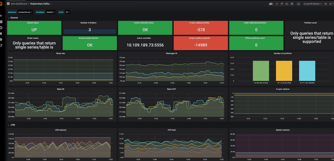
# Uninstalling Kafka Cluster
Use the following command to uninstall the Kafka cluster:
```bash
helm -n kafka uninstall kafka
```
## Deleting PVCs
Deleting PVCs will remove persistent data from the Kafka cluster. Please ensure you have backed up your data before proceeding.
```bash
kubectl -n kafka delete pvc -l app.kubernetes.io/instance=kafka
```
---
## Deploying MinIO Cluster
In this guide, you will learn how to deploy a MinIO cluster on Kubernetes using a Helm Chart.
## Prerequisites
- Kubernetes >= v1.18.0
- [kubectl](https://kubernetes.io/docs/tasks/tools/install-kubectl/) >= v1.18.0
- [Helm](https://helm.sh/docs/intro/install/) >= v3.0.0
## Configuration Management
Before installation, you need to create a `minio-values.yaml` configuration file. Please adjust the following configuration according to your Kubernetes environment:
```yaml
global:
security:
allowInsecureImages: true
image:
registry: docker.io
repository: greptime/minio
tag: 2025.4.22-debian-12-r1
auth:
rootUser: greptimedbadmin
rootPassword: "greptimedbadmin"
resources:
requests:
cpu: 500m
memory: 500Mi
limits:
cpu: '2'
memory: 2Gi
extraEnvVars:
- name: MINIO_REGION
value: "ap-southeast-1"
statefulset:
replicaCount: 4
mode: distributed
persistence:
storageClass: null
size: 100Gi
```
## Installing MinIO Cluster
Install the MinIO cluster in the minio namespace:
```bash
helm upgrade \
--install minio oci://registry-1.docker.io/bitnamicharts/minio \
--create-namespace \
--version 16.0.10 \
-n minio --values minio-values.yaml
```
Expected Output
```bash
Release "minio" does not exist. Installing it now.
Pulled: greptime-registry.cn-hangzhou.cr.aliyuncs.com/charts/minio:16.0.10
Digest: sha256:96e220fd7cf1596879a243453b39c96a95d34f0005fdd452da3d094a7b386eb4
NAME: minio
LAST DEPLOYED: Tue May 12 17:21:30 2026
NAMESPACE: minio
STATUS: deployed
REVISION: 1
TEST SUITE: None
NOTES:
CHART NAME: minio
CHART VERSION: 16.0.10
APP VERSION: 2025.4.22
Did you know there are enterprise versions of the Bitnami catalog? For enhanced secure software supply chain features, unlimited pulls from Docker, LTS support, or application customization, see Bitnami Premium or Tanzu Application Catalog. See https://www.arrow.com/globalecs/na/vendors/bitnami for more information.
** Please be patient while the chart is being deployed **
MinIO® can be accessed via port on the following DNS name from within your cluster:
minio.minio.svc.cluster.local
To get your credentials run:
export ROOT_USER=$(kubectl get secret --namespace minio minio -o jsonpath="{.data.root-user}" | base64 -d)
export ROOT_PASSWORD=$(kubectl get secret --namespace minio minio -o jsonpath="{.data.root-password}" | base64 -d)
To connect to your MinIO® server using a client:
- Run a MinIO® Client pod and append the desired command (e.g. 'admin info'):
kubectl run --namespace minio minio-client \
--rm --tty -i --restart='Never' \
--env MINIO_SERVER_ROOT_USER=$ROOT_USER \
--env MINIO_SERVER_ROOT_PASSWORD=$ROOT_PASSWORD \
--env MINIO_SERVER_HOST=minio \
--image docker.io/bitnami/minio-client:2025.4.16-debian-12-r1 -- admin info minio
To access the MinIO® web UI:
- Get the MinIO® URL:
echo "MinIO® web URL: http://127.0.0.1:9001/minio"
kubectl port-forward --namespace minio svc/minio 9001:9001
Substituted images detected:
- greptime-registry.cn-hangzhou.cr.aliyuncs.com/greptime/minio:2025.4.22-debian-12-r1
```
## Verifying MinIO Cluster Installation
Check the status of MinIO Pods:
```bash
kubectl get pod -n minio
```
Expected Output
```bash
NAME READY STATUS RESTARTS AGE
minio-0 1/1 Running 0 30s
minio-1 1/1 Running 0 30s
minio-2 1/1 Running 0 30s
minio-3 1/1 Running 0 30s
```
# Creating Bucket and Access Key
## Accessing MinIO Console
1. First, expose the MinIO console service. You can use the kubectl port-forward command:
```bash
kubectl port-forward -n minio svc/minio 9001:9001
```
2. Open your browser: http://localhost:9001/login
3. Log in using the credentials set in the configuration file:
- username: `greptimedbadmin`
- password: `greptimedbadmin`

## Creating a Bucket
After logging into the MinIO console, follow these steps to create a Bucket:
1. Click "Buckets" in the left sidebar
2. Click the "Create Bucket" button
3. Enter a Bucket name, for example:`greptimedb-bucket`
4. Click "Create Bucket" to confirm creation
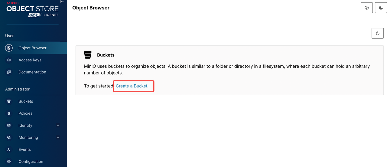
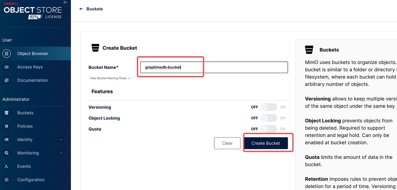
## Generating Access Key
1. Click "Access Keys" in the left sidebar
2. Click the "Create Access Key" button
3. Optional: Set permission policies
4. Click "Create" to generate the Access Key and Secret Key
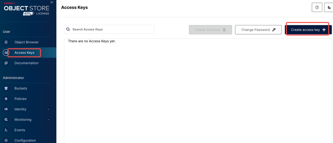
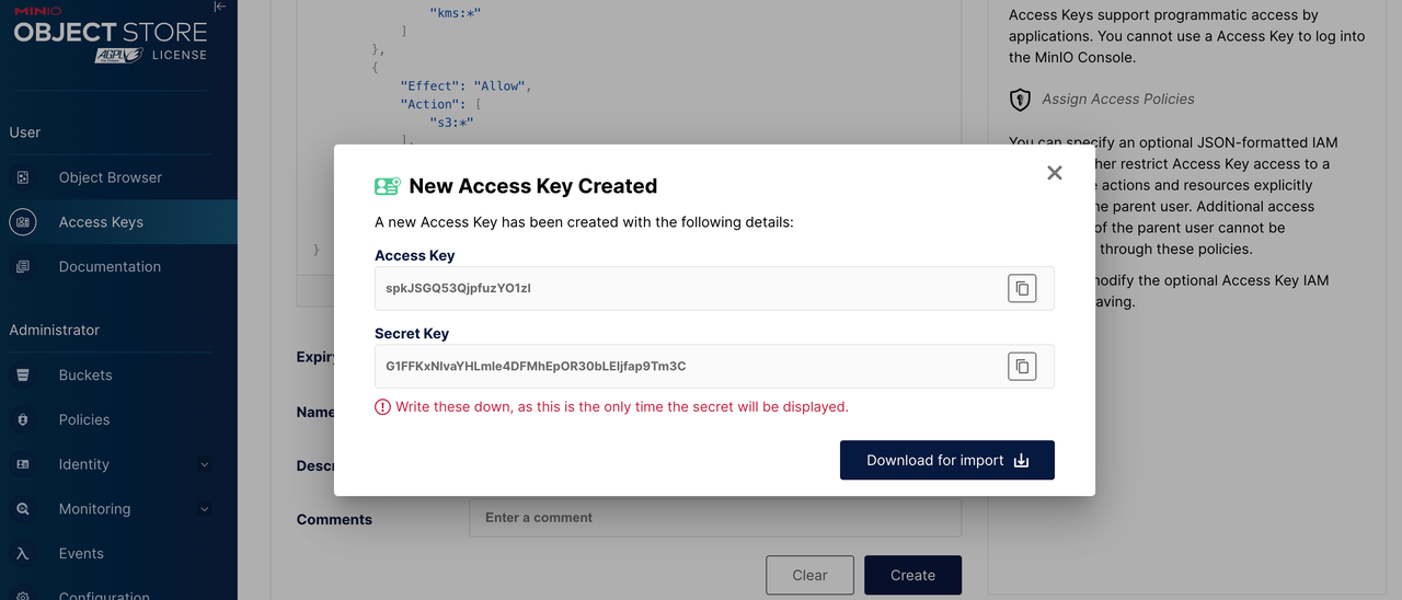
:::warning
⚠️ Important: Please save the following information securely. You will need it when deploying GreptimeDB.
- Bucket name:greptimedb-bucket
- Region:ap-southeast-1
- MinIO Endpoint:`http://minio.minio:9000`
- Access Key:The Access Key
- Secret Key:The Secret Key
:::
# Configuring GreptimeDB to Use MinIO
When deploying a GreptimeDB cluster, you can use MinIO as backend storage with the following configuration:
```yaml
objectStorage:
credentials:
accessKeyId: ""
secretAccessKey: ""
s3:
bucket: "greptimedb-bucket"
region: "ap-southeast-1"
root: "greptimedb-data"
endpoint: "http://minio.minio:9000"
```
# Monitoring
- Install Prometheus Operator (e.g: [kube-prometheus-stack](https://github.com/prometheus-community/helm-charts/tree/main/charts/kube-prometheus-stack))。
- Install podmonitor CRD。
To monitor the MinIO cluster, you need to have a monitoring system (such as Prometheus and Grafana) deployed in advance. Then add the following content to `minio-values.yaml` and re-run the command to update the MinIO configuration:
```yaml
metrics:
enabled: true
serviceMonitor:
enabled: true
namespace: minio
labels:
release: kube-prometheus-stack
interval: 30s
```
## Grafana dashboard
Use the [MinIO Dashboard](https://grafana.com/grafana/dashboards/13502-minio-dashboard/) (ID: 13502) to monitor MinIO metrics.
1. Log in to your Grafana.
2. Navigate to Dashboards -> New -> Import.
3. Enter Dashboard ID: 13502, select a data source, and load the dashboard.
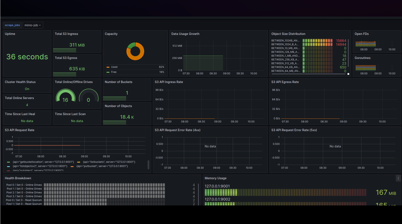
# Uninstalling MinIO Cluster
Use the following command to uninstall the MinIO cluster:
```bash
helm -n minio uninstall minio
```
## Deleting PVCs
Deleting PVCs will remove persistent data from the MinIO cluster. Please ensure you have backed up your data before proceeding.
```bash
kubectl -n minio delete pvc -l app.kubernetes.io/instance=minio
```
---
## GreptimeDB Operator Management
The GreptimeDB Operator manages the [GreptimeDB](https://github.com/GrepTimeTeam/greptimedb) resources on [Kubernetes](https://kubernetes.io/) using the [Operator pattern](https://kubernetes.io/docs/concepts/extend-kubernetes/operator/).
It is like an autopilot that automates the deployment, provisioning, and orchestration of the GreptimeDB cluster and standalone.
The GreptimeDB Operator includes, but is not limited to, the following features:
- **Automated Provisioning**: Automates the deployment of the GreptimeDB cluster and standalone on Kubernetes by providing CRD `GreptimeDBCluster` and `GreptimeDBStandalone`.
- **Multi-Cloud Support**: Users can deploy the GreptimeDB on any Kubernetes cluster, including on-premises and cloud environments(like AWS, GCP, Aliyun, etc.).
- **Scaling**: Scale the GreptimeDB cluster as easily as changing the `replicas` field in the `GreptimeDBCluster` CR.
- **Monitoring Bootstrap**: Bootstrap the GreptimeDB monitoring stack for the GreptimeDB cluster by providing the `monitoring` field in the `GreptimeDBCluster` CR.
This document will show you how to install, upgrade, configure, and uninstall the GreptimeDB Operator on Kubernetes.
:::note
The following output may have minor differences depending on the versions of the Helm charts and environment.
:::
## Prerequisites
- Kubernetes >= v1.18.0
- [kubectl](https://kubernetes.io/docs/tasks/tools/install-kubectl/) >= v1.18.0
- [Helm](https://helm.sh/docs/intro/install/) >= v3.0.0
## Production Deployment
For production deployments, it's recommended to use Helm to install the GreptimeDB Operator.
### Installation
You can refer [Install and verify the GreptimeDB Operator](/user-guide/deployments-administration/deploy-on-kubernetes/deploy-greptimedb-cluster.md#install-and-verify-the-greptimedb-operator) for detailed instructions.
:::note
If you are using [Argo CD](https://argo-cd.readthedocs.io/en/stable/) to deploy applications, please make sure that the `Application` has set the [`ServerSideApply=true`](https://argo-cd.readthedocs.io/en/latest/user-guide/sync-options/#server-side-apply) to enable the server-side apply (other GitOps tools may have similar settings).
:::
### Upgrade
We always publish the latest version of the GreptimeDB Operator as a Helm chart in our official Helm repository.
When the new version of the GreptimeDB Operator is released, you can upgrade the GreptimeDB Operator by running the following commands.
#### Update the Helm repository
```bash
helm repo update greptime
```
Expected Output
```bash
Hang tight while we grab the latest from your chart repositories...
...Successfully got an update from the "greptime" chart repository
Update Complete. ⎈Happy Helming!⎈
```
You can use the following command to search the latest version of the GreptimeDB Operator:
```bash
helm search repo greptime/greptimedb-operator
```
Expected Output
```bash
NAME CHART VERSION APP VERSION DESCRIPTION
greptime/greptimedb-operator 0.5.9 0.5.5 The greptimedb-operator Helm chart for Kubernetes.
```
You also can use the following command to list all the available versions:
```bash
helm search repo greptime/greptimedb-operator --versions
```
#### Upgrade the GreptimeDB Operator
You can upgrade to the latest released version of the GreptimeDB Operator by running the following command:
```bash
helm -n greptimedb-admin upgrade --install greptimedb-operator greptime/greptimedb-operator
```
Expected Output
```bash
NAME: greptimedb-operator
LAST DEPLOYED: Sun Apr 26 20:43:58 2026
NAMESPACE: greptimedb-admin
STATUS: deployed
REVISION: 1
TEST SUITE: None
NOTES:
***********************************************************************
Welcome to use greptimedb-operator
Chart version: 0.5.9
GreptimeDB Operator version: 0.5.5
***********************************************************************
Installed components:
* greptimedb-operator
The greptimedb-operator is starting, use `kubectl get deployment greptimedb-operator -n greptimedb-admin` to check its status.
```
If you want to upgrade to a specific version, you can use the following command:
```bash
helm -n greptimedb-admin upgrade --install greptimedb-operator greptime/greptimedb-operator --version
```
After the upgrade is complete, you can use the following command to verify the installation:
```bash
helm list -n greptimedb-admin
```
Expected Output
```bash
NAME NAMESPACE REVISION UPDATED STATUS CHART APP VERSION
greptimedb-operator greptimedb-admin 1 2026-04-26 20:43:58.003167 +0800 CST deployed greptimedb-operator-0.5.9 0.5.5
```
### CRDs
There are two kinds of CRD that are installed with the GreptimeDB Operator: `GreptimeDBCluster` and `GreptimeDBStandalone`.
You can use the following command to verify the installation:
```bash
kubectl get crd | grep greptime
```
Expected Output
```bash
greptimedbclusters.greptime.io 2026-04-26T12:43:58Z
greptimedbstandalones.greptime.io 2026-04-26T12:43:58Z
```
By default, the GreptimeDB Operator chart will manage the installation and upgrade of the CRDs and the users don't need to manage them manually. If you want to know the specific definitions of these two types of CRD, you can refer to the GreptimeDB Operator [API documentation](https://github.com/GreptimeTeam/greptimedb-operator/blob/main/docs/api-references/docs.md).
### Configuration
The GreptimeDB Operator chart provides a set of configuration options that allow you to customize the installation, you can refer to the [GreptimeDB Operator Helm Chart](https://github.com/GreptimeTeam/helm-charts/blob/main/charts/greptimedb-operator/README.md##values) for more details.
You can create a `values.yaml` to configure the GreptimeDB Operator chart (the complete configuration of `values.yaml` can be found in the [chart](https://github.com/GreptimeTeam/helm-charts/blob/main/charts/greptimedb-operator/values.yaml)), for example:
```yaml
image:
# -- The image registry
registry: docker.io
# -- The image repository
repository: greptime/greptimedb-operator
# -- The image pull policy for the controller
imagePullPolicy: IfNotPresent
# -- The image tag
tag: "v0.5.6"
# -- The image pull secrets
pullSecrets: []
replicas: 1
resources:
limits:
cpu: 500m
memory: 512Mi
requests:
cpu: 250m
memory: 256Mi
```
You also can use one command to install or upgrade the GreptimeDB Operator with the custom configuration:
```bash
helm -n greptimedb-admin upgrade --install greptimedb-operator greptime/greptimedb-operator -f values.yaml
```
### Uninstallation
You can use the `helm` command to uninstall the GreptimeDB Operator:
```bash
helm -n greptimedb-admin uninstall greptimedb-operator
```
We don't delete the CRDs by default when you uninstall the GreptimeDB Operator.
:::danger
If you really want to delete the CRDs, you can use the following command:
```bash
kubectl delete crd greptimedbclusters.greptime.io greptimedbstandalones.greptime.io
```
The related resources will be removed after you delete the CRDs.
:::
---
## Deploy GreptimeDB on Kubernetes
GreptimeDB is designed for cloud-native environments and supports Kubernetes deployment from day one.
You can deploy GreptimeDB on any cloud service provider, including AWS, Alibaba Cloud, or Google Cloud.
## Deploy GreptimeDB Standalone
For development, testing, or small-scale production use cases, you can [deploy a standalone GreptimeDB instance](deploy-greptimedb-standalone.md) on Kubernetes.
This provides a simple way to get started with GreptimeDB without the complexity of managing a full cluster.
## Deploy GreptimeDB Cluster
For production environments requiring high availability and scalability,
you can [deploy a GreptimeDB cluster](deploy-greptimedb-cluster.md) using the GreptimeDB Operator on Kubernetes.
This enables you to set up a distributed GreptimeDB cluster that scales horizontally and efficiently handles large volumes of data.
## Configurations
You can apply custom configurations to GreptimeDB by creating a `values.yaml` file
when deploying either GreptimeDB clusters or standalone instances.
For a complete list of available configuration options, see [Common Helm Chart Configurations](./common-helm-chart-configurations.md).
## Manage GreptimeDB Operator
The GreptimeDB Operator manages GreptimeDB deployments on Kubernetes,
automating the setup, provisioning, and management of GreptimeDB cluster instances.
This enables quick deployment and scaling of GreptimeDB in any Kubernetes environment,
whether on-premises or in the cloud.
Learn how to [manage the GreptimeDB Operator](./greptimedb-operator-management.md),
including installation and upgrades.
## Advanced Deployments
After familiarizing yourself with [the architecture and components of GreptimeDB](/user-guide/concepts/architecture.md), you can explore advanced deployment scenarios:
- [Deploy GreptimeDB Infrastructure test](deploy-greptimedb-infra-test.md): Prerequisite infrastructure testing for installing GreptimeDB.
- [Deploy MinIO cluster](deploy-minio.md):Learn how to deploy, configure, and monitor a MinIO cluster.
- [Deploy Kafka cluster](deploy-kafka.md):Learn how to deploy, configure, and monitor a Kafka cluster.
- [Deploy GreptimeDB Cluster with Remote WAL](configure-remote-wal.md): Configure Kafka as a remote write-ahead log (WAL) for your GreptimeDB cluster to persistently record every data modification and ensure no loss of memory-cached data.
- [Use MySQL/PostgreSQL as Metadata Store](/user-guide/deployments-administration/deploy-on-kubernetes/common-helm-chart-configurations.md#configuring-metasrv-backend-storage): Integrate MySQL/PostgreSQL databases to provide robust metadata storage capabilities for enhanced reliability and performance.
- [Deploy Multi-Frontend GreptimeDB Cluster](configure-frontend-groups.md): Set up a GreptimeDB cluster on Kubernetes with a frontend group consisting of multiple frontend instances for improved load distribution and availability.
---
## Data Export & Import
This guide describes how to use GreptimeDB's Export and Import tools for database data backup and restoration operations.
For detailed command-line options and advanced configurations, please refer to [Data Export & Import](/reference/command-lines/utilities/data.md).
## Overview
## Export Operations
### Full Databases Backup
Export all databases backup. This operation exports each database into a single directory, including all tables and their data.
```bash
# Export all databases backup
greptime cli data export \
--addr localhost:4000 \
--output-dir /tmp/backup/greptimedb
```
The output directory structure is as follows:
```
/
└── greptime/
└── /
├── create_database.sql
├── create_tables.sql
├── copy_from.sql
└──
```
#### Export to S3
Export all databases backup to S3:
```bash
greptime cli data export \
--addr localhost:4000 \
--s3 \
--s3-bucket \
--s3-access-key-id \
--s3-secret-access-key \
--s3-region \
--s3-root \
--s3-endpoint
```
### Export with Basic Authentication
If the GreptimeDB instance has authentication enabled, pass the credentials with `--auth-basic`:
```bash
greptime cli data export \
--addr localhost:4000 \
--output-dir /tmp/backup/greptimedb \
--auth-basic :
```
### Schema-Only Operations
Export only schemas without data. This operation exports `CREATE TABLE` statements into SQL files, allowing you to backup table structures without the actual data.
```bash
# Export only schemas
greptime cli data export \
--addr localhost:4000 \
--output-dir /tmp/backup/schemas \
--target schema
```
### Time-Range Based Backup
```bash
# Export data within specific time range
greptime cli data export --addr localhost:4000 \
--output-dir /tmp/backup/timerange \
--start-time "2024-01-01 00:00:00" \
--end-time "2024-01-31 23:59:59"
```
### Specific Database Backup
```bash
# To export a specific database
greptime cli data export \
--addr localhost:4000 \
--output-dir /tmp/backup/greptimedb \
--database '{my_database_name}'
```
## Import Operations
### Full Databases Backup
Import all databases backup.
```bash
# Import all databases
greptime cli data import \
--addr localhost:4000 \
--input-dir /tmp/backup/greptimedb
```
### Import with Basic Authentication
If the GreptimeDB instance has authentication enabled, pass the credentials with `--auth-basic`:
```bash
greptime cli data import \
--addr localhost:4000 \
--input-dir /tmp/backup/greptimedb \
--auth-basic :
```
### Schema-Only Operations
Import only schemas without data. This operation imports `CREATE TABLE` statements from SQL files, allowing you to restore table structures without the actual data.
```bash
# Import only schemas
greptime cli data import \
--addr localhost:4000 \
--input-dir /tmp/backup/schemas \
--target schema
```
### Specific Database Backup
```bash
# The same applies to import tool
greptime cli data import \
--addr localhost:4000 \
--input-dir /tmp/backup/greptimedb \
--database '{my_database_name}'
```
## Best Practices
1. **Parallelism Configuration**
- Adjust `--export-jobs`/`--import-jobs` based on available system resources
- Start with a lower value and increase gradually
- Monitor system performance during operations
2. **Backup Strategy**
- Incremental data backups using time ranges
- Periodic backups for disaster recovery
3. **Error Handling**
- Use `--max-retry` for handling transient failures
- Keep logs for troubleshooting
## Performance Tips
1. **Export Performance**
- Use time ranges for large datasets
- Adjust parallel jobs based on CPU/Memory
- Consider network bandwidth limitations
2. **Import Performance**
- Monitor database resources
## Troubleshooting
1. **Connection Errors**
- Verify server address and port
- Check network connectivity
- Ensure authentication credentials are correct
2. **Permission Issues**
- Verify read/write permissions on output/input directories
3. **Resource Constraints**
- Reduce parallel jobs
- Ensure sufficient disk space
- Monitor system resources during operations
---
## Metadata Export & Import
This guide describes how to use GreptimeDB's metadata export and import tools for metadata backup and restoration operations.
For detailed command-line options and advanced configurations, please refer to [Metadata Export & Import](/reference/command-lines/utilities/metadata.md).
## Overview
## Export Operations
### Export to S3 Cloud Storage
Export metadata from PostgreSQL to S3 for cloud-based backup storage:
```bash
greptime cli meta snapshot save \
--store-addrs 'password=password dbname=postgres user=postgres host=localhost port=5432' \
--backend postgres-store \
--s3 \
--s3-bucket your-bucket-name \
--s3-region ap-southeast-1 \
--s3-access-key-id \
--s3-secret-access-key
```
**Output**: Creates `metadata_snapshot.metadata.fb` file in the specified S3 bucket.
### Export to Local Directory
#### From PostgreSQL Backend
Export metadata from PostgreSQL to local directory:
```bash
greptime cli meta snapshot save \
--store-addrs 'password=password dbname=postgres user=postgres host=localhost port=5432' \
--backend postgres-store
```
#### From MySQL Backend
Export metadata from MySQL to local directory:
```bash
greptime cli meta snapshot save \
--store-addrs 'mysql://user:password@127.0.0.1:3306/database' \
--backend mysql-store
```
#### From etcd Backend
Export metadata from etcd to local directory:
```bash
greptime cli meta snapshot save \
--store-addrs 127.0.0.1:2379 \
--backend etcd-store
```
**Output**: Creates `metadata_snapshot.metadata.fb` file in the current working directory.
#### From RaftEngine Backend
:::note
RaftEngine locks the metadata directory while the standalone instance is running. Stop the standalone instance before exporting.
:::
Export metadata from RaftEngine to local directory:
```bash
greptime cli meta snapshot save \
--store-addrs "raftengine:///path/to/metadata" \
--backend raft-engine-store
```
**Output**: Creates `metadata_snapshot.metadata.fb` file in the current working directory.
## Import Operations
:::warning
**Important**: Before importing metadata, ensure the target backend is in a **clean state** (contains no existing data). Importing to a non-empty backend may result in data corruption or conflicts.
If you need to import to a backend with existing data, use the `--force` flag to bypass this safety check. However, exercise extreme caution as this can lead to data loss or inconsistencies.
:::
### Import from S3 Cloud Storage
Restore metadata from S3 backup to PostgreSQL storage backend:
```bash
greptime cli meta snapshot restore \
--store-addrs 'password=password dbname=postgres user=postgres host=localhost port=5432' \
--backend postgres-store \
--s3 \
--s3-bucket your-bucket-name \
--s3-region ap-southeast-1 \
--s3-access-key-id \
--s3-secret-access-key
```
### Import from Local File
#### To PostgreSQL Backend
Restore metadata from local backup file to PostgreSQL:
```bash
greptime cli meta snapshot restore \
--store-addrs 'password=password dbname=postgres user=postgres host=localhost port=5432' \
--backend postgres-store
```
#### To MySQL Backend
Restore metadata from local backup file to MySQL:
```bash
greptime cli meta snapshot restore \
--store-addrs 'mysql://user:password@127.0.0.1:3306/database' \
--backend mysql-store
```
#### To etcd Backend
Restore metadata from local backup file to etcd:
```bash
greptime cli meta snapshot restore \
--store-addrs 127.0.0.1:2379 \
--backend etcd-store
```
#### To RaftEngine Backend
Restore metadata from local backup file to RaftEngine:
```bash
greptime cli meta snapshot restore \
--store-addrs "raftengine:///path/to/metadata" \
--backend raft-engine-store
```
---
## DR Solution Based on Cross-Region Deployment in a Single Cluster
## How disaster recovery works in GreptimeDB
GreptimeDB is well-suited for cross-region disaster recovery. You may have varying regional characteristics and business needs, and GreptimeDB offers tailored solutions to meet these diverse requirements.
GreptimeDB resource management involves the concept of Availability Zones (AZs). An AZ is a logical unit of disaster recovery.
It can be a Data Center (DC), a compartment of a DC. This depends on your specific DC conditions and deployment design.
In the cross region disaster recovery solutions, a GreptimeDB region is a city. When two DC are in the same region and one DC becomes unavailable, the other DC can take over the services of the unavailable DC. This is a localization strategy.
Before understanding the details of each DR solution, it is necessary to first understand the following knowledge:
1. The DR solution for the remote wal component is also very important. Essentially, it forms the foundation of the entire DR solution. Therefore, for each DR solution of GreptimeDB, we will let the remote wal component in the diagram. Currently, GreptimeDB's default remote wal component is implemented based on Kafka, and other implementations will be provided in the future; however, there won't be significant differences in deployment.
2. The table of GreptimeDB: Each table can be divided into multiple partitions according to a certain range, and each partition may be distributed on different datanodes. When writing or querying, the specified node will be called according to the corresponding rules. A table's partitions might look like this:
```
Table name: T1
Table partition count: 4
T1-1
T1-2
T1-3
T1-4
Table name: T2
Table partition count: 3
T2-1
T2-2
T2-3
```
### Metadata across 2 regions, data in the same region

In this solution, the data is in one region (2 DCs), while the metadata across 2 regions.
DC1 and DC2 are used together to handle read and write services, while DC3 (located in region2) is a replica used to meet the majority protocol. This architecture is also called the "2-2-1" solution.
Both DC1 and DC2 must be able to handle all requests in extreme situations, so please ensure that sufficient resources are allocated.
Latencies:
- 2ms latency in the same region
- 30ms latency in two regions
Supports High Availability:
- A single AZ is unavailable with the same performance
- A single DC is unavailable with almost the same performance
If you want a regional-level disaster recovery solution, you can take it a step further by providing read and write services on DC3. So, the next solution is:
### Data across 2 regions
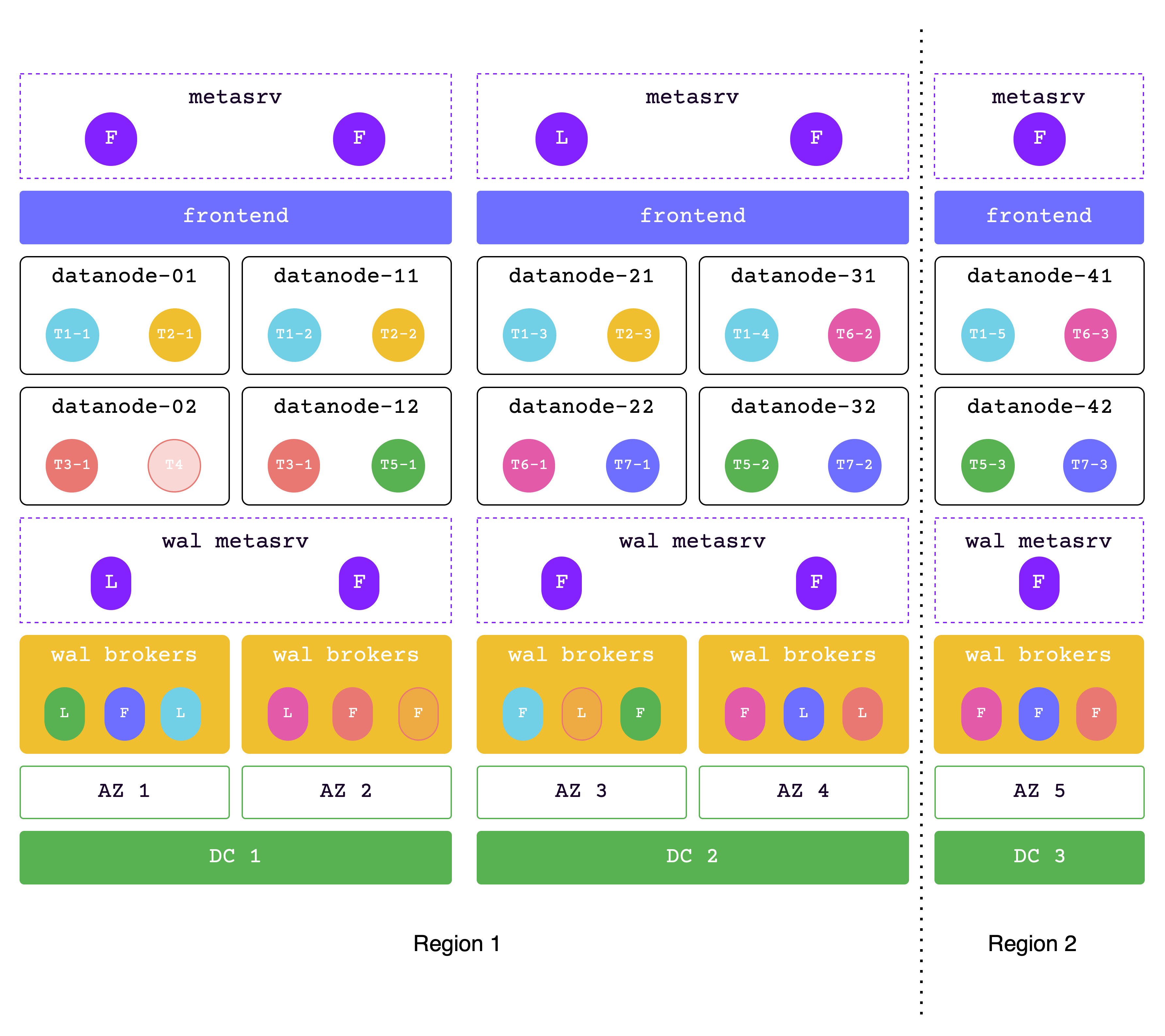
In this solution, the data across 2 regions.
Each DC must be able to handle all requests in extreme situations, so please ensure that sufficient resources are allocated.
Latencies:
- 2ms latency in the same region
- 30ms latency in two regions
Supports High Availability:
- A single AZ is unavailable with the same performance
- A single DC is unavailable with degraded performance
If you can't tolerate performance degradation from a single DC failure, consider upgrading to the five-DC and three-region solution.
### Metadata across 3 regions, data across 2 regions
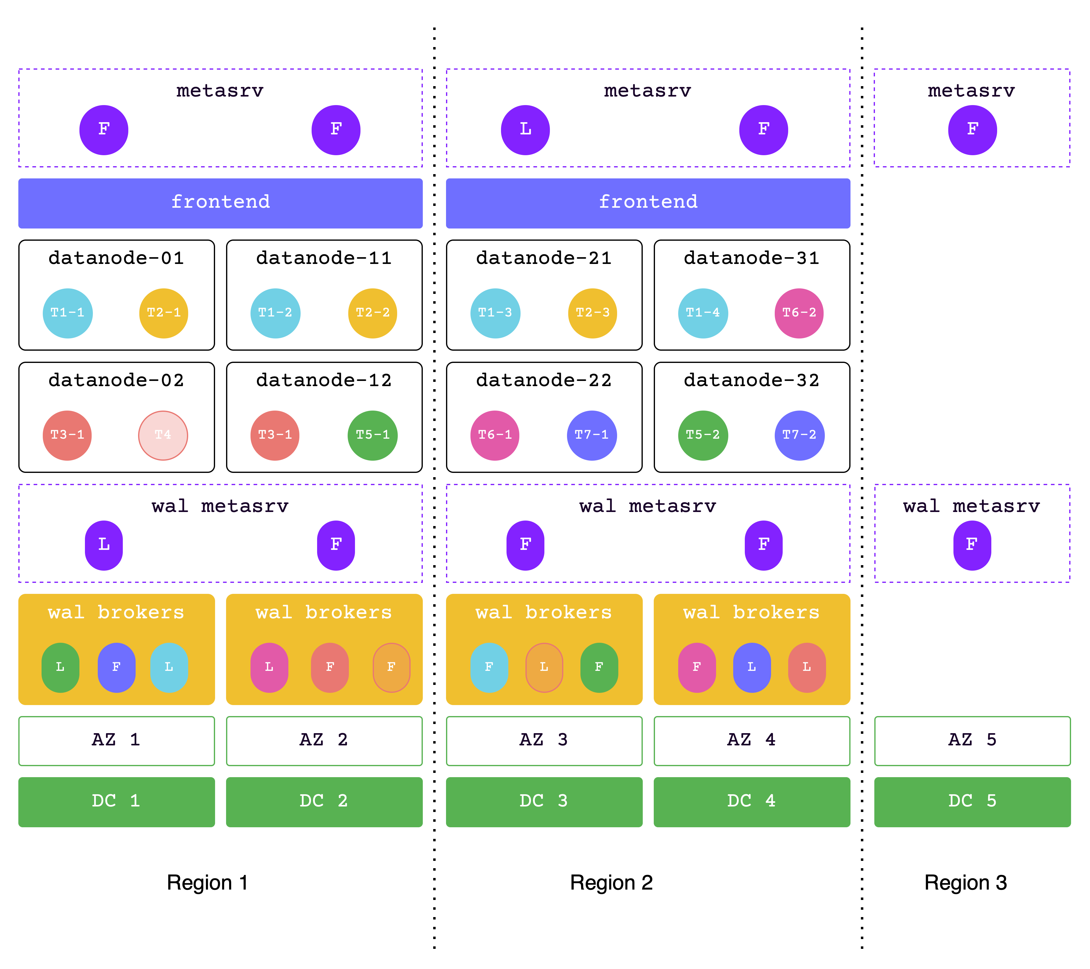
In this solution, the data across 2 regions, while the metadata across 3 regions.
Region1 and region2 are used together to handle read and write services, while region3 is a replica used to meet the majority protocol. This architecture is also called the "2-2-1" solution.
Each of the two adjacent regions must be able to handle all requests in extreme situations, so please ensure that sufficient resources are allocated.
Latencies:
- 2ms latency in the same region
- 7ms latency in two adjacent regions
- 30ms latency in two distant regions
Supports High Availability:
- A single AZ is unavailable with the same performance
- A single DC is unavailable with the same performance
- A single region(city) is unavailable with slightly degraded performance
You can take it a step further by providing read and write services on both 3 regions. So, the next solution is:
(This solution may have higher latency, so if that's unacceptable, it's not recommended.)
### Data across 3 regions
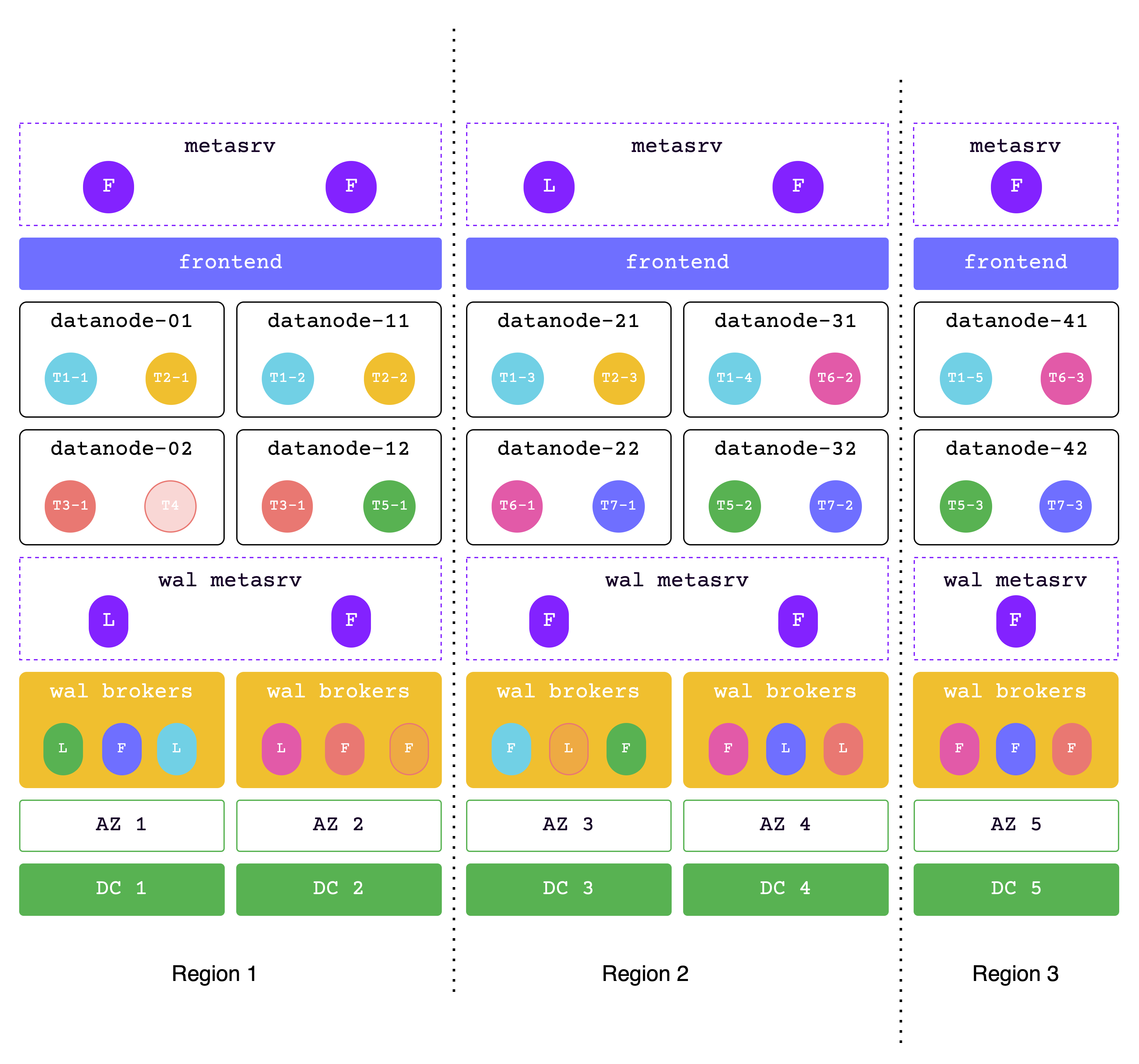
In this solution, the data across 3 regions.
In the event of a failure in one region, the other two regions must be able to handle all requests, so please ensure sufficient resources are allocated.
Latencies:
- 2ms latency in the same region
- 7ms latency in two adjacent regions
- 30ms latency in two distant regions
Supports High Availability:
- A single AZ is unavailable with the same performance
- A single DC is unavailable with the same performance
- A single region(city) is unavailable with degraded performance
## Solution Comparison
The goal of the above solutions is to meet the high requirements for availability and reliability in medium to large-scale scenarios. However, in specific implementations, the cost and effectiveness of each solution may vary. The table below compares each solution to help you choose the final plan based on your specific scenario, needs, and costs.
Here is the content formatted into a table:
| Solution | Latencies | High Availability |
| --- | --- | --- |
| Metadata across 2 regions, data in the same region | - 2ms latency in the same region- 30ms latency in two regions | - A single AZ is unavailable with the same performance- A single DC is unavailable with almost the same performance |
| Data across 2 regions | - 2ms latency in the same region- 30ms latency in two regions | - A single AZ is unavailable with the same performance- A single DC is unavailable with degraded performance |
| Metadata across 3 regions, data across 2 regions | - 2ms latency in the same region- 7ms latency in two adjacent regions- 30ms latency in two distant regions | - A single AZ is unavailable with the same performance- A single DC is unavailable with the same performance- A single region(city) is unavailable with slightly degraded performance |
| Data across 3 regions | - 2ms latency in the same region- 7ms latency in two adjacent regions- 30ms latency in two distant regions | - A single AZ is unavailable with the same performance - A single DC is unavailable with the same performance- A single region(city) is unavailable with degraded performance |
---
## DR solution for GreptimeDB Standalone
---
## Disaster Recovery
GreptimeDB is a distributed database designed to withstand disasters. It provides different solutions for disaster recovery (DR).
This document contains:
* Basic concepts in DR.
* The deployment architecture of GreptimeDB and Backup & Restore (BR).
* GreptimeDB provides the DR solutions.
* Compares these DR solutions.
## Basic Concepts
* **Recovery Time Objective (RTO)**: refers to the maximum acceptable amount of time that a business process can be down after a disaster occurs before it negatively impacts the organization.
* **Recovery Point Objective (RPO)**: refers to the maximum acceptable amount of time since the last data recovery point. This determines what is considered an acceptable loss of data between the last recovery point and the interruption of service.
The following figure illustrates these two concepts:
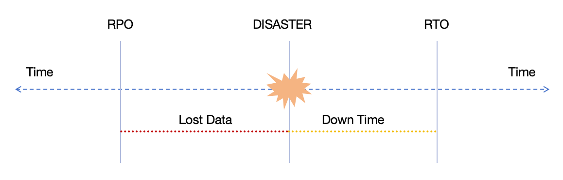
* **Write-Ahead Logging (WAL)**: persistently records every data modification to ensure data integrity and consistency.
GreptimeDB storage engine is a typical [LSM Tree](https://en.wikipedia.org/wiki/Log-structured_merge-tree) :
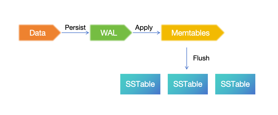
The data written is going firstly persisted into WAL, then applied into Memtable in memory. Under specific conditions (e.g., exceeding the memory threshold), the Memtable will be flushed and persisted as an SSTable. So the DR of WAL and SSTable is key to the DR of GreptimeDB.
* **Region**: a contiguous segment of a table, and also could be regarded as a partition in some relational databases. Read [Table Sharding](/contributor-guide/frontend/table-sharding.md#region) for more details.
## Component architecture
### GreptimeDB
Before digging into the specific DR solution, let's explain the architecture of GreptimeDB components in the perspective of DR:
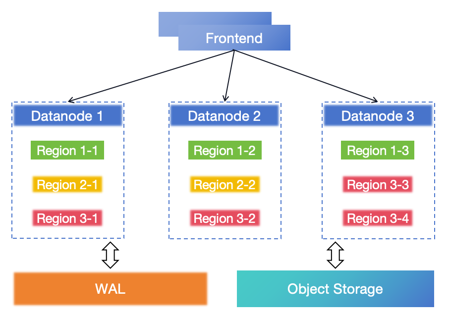
GreptimeDB is designed with a cloud-native architecture based on storage-compute separation:
* **Frontend**: the ingestion and query service layer, which forwards requests to Datanode and processes, and merges responses from Datanode.
* **Datanode**: the storage layer of GreptimeDB, and is an LSM storage engine. Region is the basic unit for storing and scheduling data in Datanode. A region is a table partition, a collection of data rows. The data in region is saved into Object Storage (such as AWS S3). Unflushed Memtable data is written into WAL and can be recovered in DR.
* **WAL**: persists the unflushed Memtable data in memory. It will be truncated when the Memtable is flushed into SSTable files. It can be local disk-based (local WAL) or Kafka cluster-based (remote WAL).
* **Object Storage**: persists the SSTable data and index.
The GreptimeDB stores data in object storage such as [AWS S3](https://docs.aws.amazon.com/AmazonS3/latest/userguide/DataDurability.html) or its compatible services, which is designed to provide 99.999999999% durability and 99.99% availability of objects over a given year. And services such as S3 provide [replications in Single-Region or Cross-Region](https://docs.aws.amazon.com/AmazonS3/latest/userguide/replication.html), which is naturally capable of DR.
At the same time, the WAL component is pluggable, e.g. using Kafka as the WAL service that offers a mature [DR solution](https://www.confluent.io/blog/disaster-recovery-multi-datacenter-apache-kafka-deployments/).
### Backup and restore
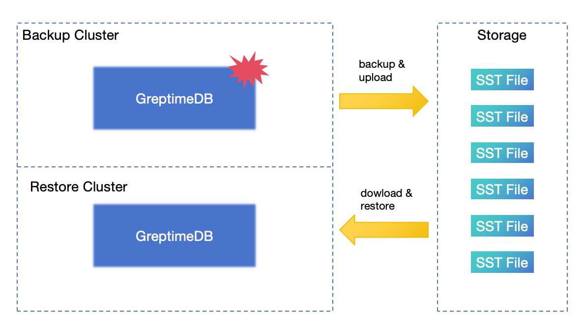
The Backup & Restore (BR) tool can perform a full snapshot backup of databases or tables at a specific time and supports incremental backup.
When a cluster encounters a disaster, you can restore the cluster from backup data. Generally speaking, BR is the last resort for disaster recovery.
## Solutions introduction
### DR solution for GreptimeDB Standalone
If the Standalone is running on the local disk for WAL and data, then:
* RPO: depends on backup frequency.
* RTO: doesn't make sense in standalone mode, mostly depends on the size of the data to be restored, your failure response time, and the operational infrastructure.
A good start is to deploy GreptimeDB Standalone into an IaaS platform that has a backup and recovery solution. For example, Amazon EC2 with EBS volumes provides a comprehensive [Backup and Recovery solution](https://docs.aws.amazon.com/prescriptive-guidance/latest/backup-recovery/backup-recovery-ec2-ebs.html).
But if running the Standalone with remote WAL and object storage, there is a better DR solution:
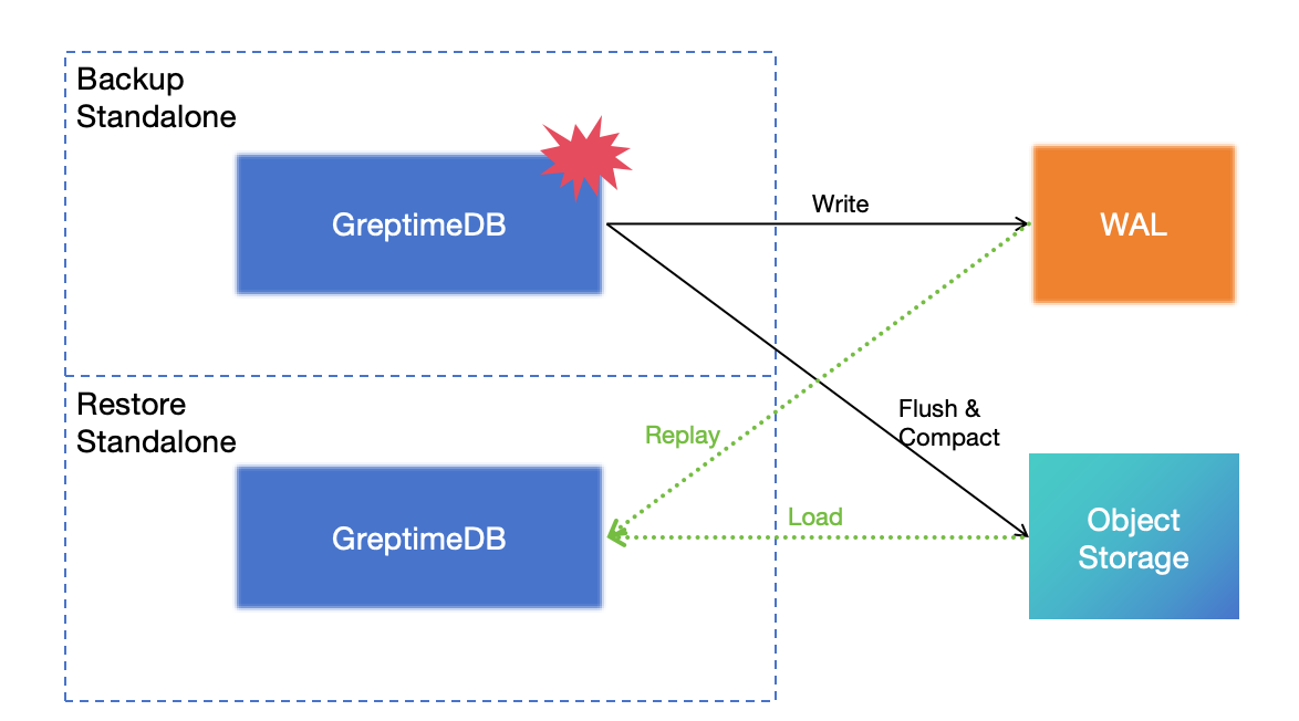
Write the WAL to the Kafka cluster and store the data in object storage, so the database itself is stateless. In the event of a disaster affecting the standalone database, you can restore it using the remote WAL and object storage. This solution can achieve **RPO=0** and **RTO in minutes**.
### DR solution based on Active-Active Failover
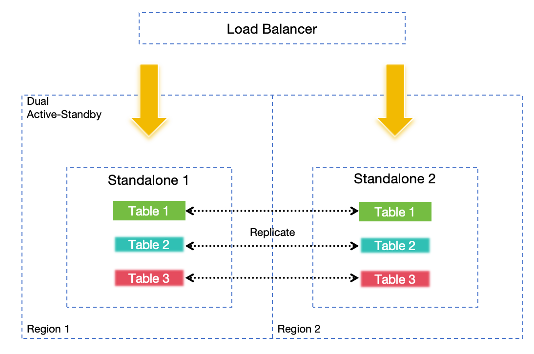
In some edge or small-to-medium scale scenarios, or if you lack the resources to deploy remote WAL or object storage, Active-Active Failover offers a better solution compared to Standalone DR. By replicating requests synchronously between two actively serving standalone nodes, high availability is ensured. The failure of any single node will not lead to data loss or a decrease in service availability even when using local disk-based WAL and data storage.
Deploying nodes in different regions can also meet region-level DR requirements, but the scalability is limited.
:::tip NOTE
**Active-Active Failover is only available in GreptimeDB Enterprise.**
:::
For more information about this solution, see [DR solution based on Active-Active Failover](/enterprise/deployments-administration/disaster-recovery/dr-solution-based-on-active-active-failover.md).
### DR solution based on cross-region deployment in a single cluster
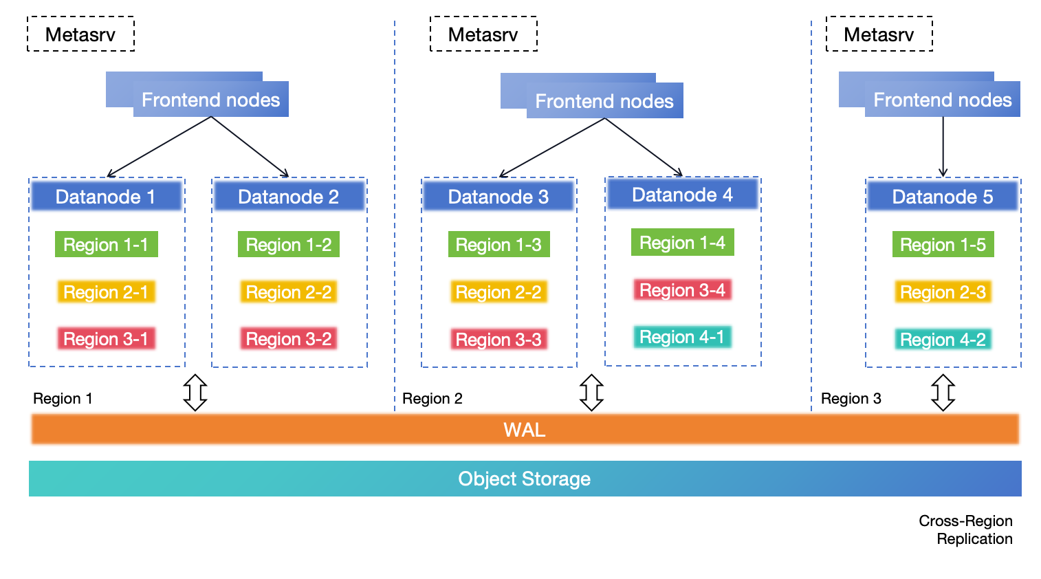
For medium-to-large scale scenarios requiring zero RPO, this solution is highly recommended. In this deployment architecture, the entire cluster spans across three regions, with each region capable of handling both read and write requests. Data replication is achieved using remote WAL and object storage, both of which must have cross-region DR enabled.
If Region 1 becomes completely unavailable due to a disaster, the table regions within it will be opened and recovered in the other regions.
In the event that Region 1 becomes completely unavailable due to a disaster, the table regions within it will be opened and recovered in the other regions. Region 3 serves as a replica to adhere to the majority protocol of Metasrv.
This solution provides region-level error tolerance, scalable write capability, zero RPO, and minute-level RTO or even lower. For more information about this solution, see [DR solution based on cross-region deployment in a single cluster](./dr-solution-based-on-cross-region-deployment-in-single-cluster.md).
### DR solution based on BR
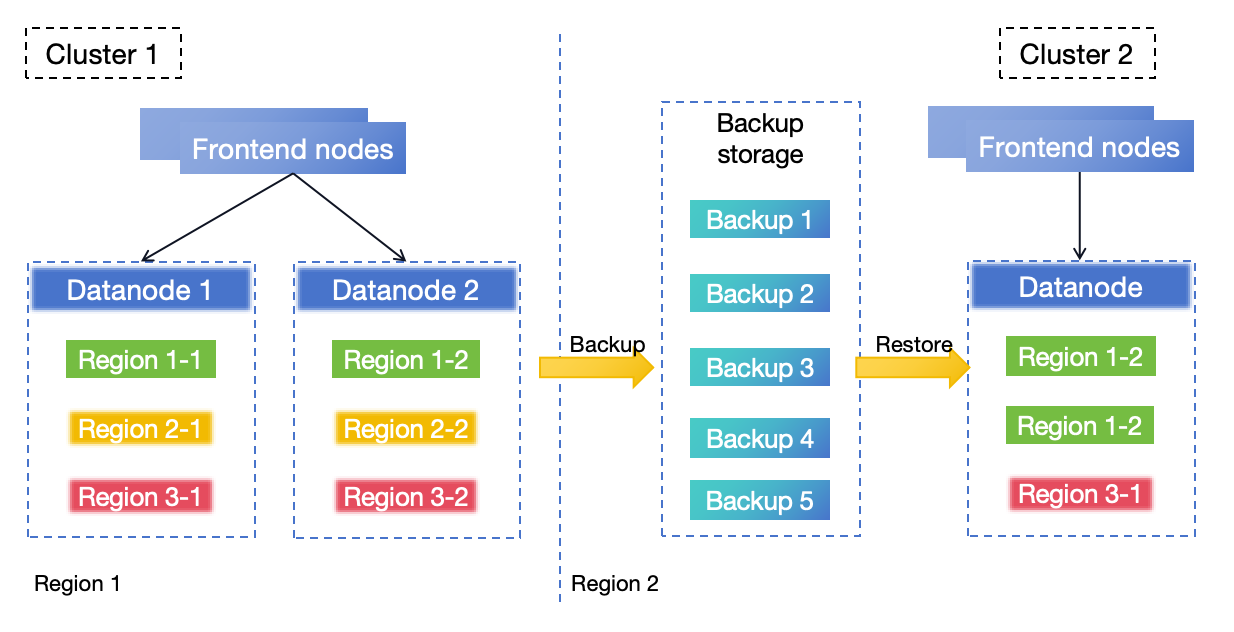
In this architecture, GreptimeDB Cluster 1 is deployed in region 1. The BR process continuously and regularly backs up the data from Cluster 1 to region 2. If region 1 experiences a disaster rendering Cluster 1 unrecoverable, you can use the backup data to restore a new cluster (Cluster 2) in region 2 to resume services.
The DR solution based on BR provides an RPO depending on the backup frequency and an RTO that varies with the size of the data to be restored.
Read [Backup & restore data](./back-up-&-restore-data.md) for details.
### Solution Comparison
By comparing these DR solutions, you can decide on the final option based on their specific scenarios, requirements, and cost.
| DR solution | Error Tolerance Objective | RPO | RTO | TCO | Scenarios | Remote WAL & Object Storage | Notes |
| ------------- | ------------------------- | ----- | ----- | ----- | ---------------- | --------- | --------|
| DR solution for Standalone| Single-Region | Backup Interval | Minute or Hour level | Low | Low requirements for availability and reliability in small scenarios | Optional | |
| DR solution based on Active-Active Failover | Cross-Region | Configurable | Minute level | Low | High requirements for availability and reliability in small-to-medium scenarios | Optional | Commercial feature |
| DR solution based on cross-region deployment in a single cluster| Multi-Regions | 0 | Minute level | High | High requirements for availability and reliability in medium-to-large scenarios | Required | |
| DR solution based on BR | Single-Region | Backup Interval | Minute or Hour level | Low | Acceptable requirements for availability and reliability | Optional | |
## References
* [Backup & restore data](./back-up-&-restore-data.md)
* [DR solution based on Active-Active Failover ](/enterprise/deployments-administration/disaster-recovery/dr-solution-based-on-active-active-failover.md)
* [DR solution based on cross-region deployment in a single cluster](./dr-solution-based-on-cross-region-deployment-in-single-cluster.md)
* [S3 Replicating objects overview](https://docs.aws.amazon.com/AmazonS3/latest/userguide/replication.html)
---
## Cluster Maintenance Mode
Maintenance mode is a safety feature in GreptimeDB that temporarily disables automatic cluster management operations.
This mode is particularly useful during:
- Cluster deployment
- Cluster upgrades
- Planned downtime
- Any operation that might temporarily affect cluster stability
## When to Use Maintenance Mode
### With GreptimeDB Operator
If you are upgrading a cluster using GreptimeDB Operator, you don't need to enable the maintenance mode manually. The operator handles this automatically.
### Without GreptimeDB Operator
When upgrading a cluster without using GreptimeDB Operator, **you must manually enable Metasrv's maintenance mode before**:
1. Deploying a new cluster (maintenance mode should be enabled after metasrv nodes are ready)
2. Rolling upgrades of Datanode nodes
3. Metasrv nodes upgrades
4. Frontend nodes upgrades
5. Any operation that might cause temporary node unavailability
After the cluster is deployed/upgraded, you can disable the maintenance mode.
## Impact of Maintenance Mode
When maintenance mode is enabled:
- Auto Balancing (if enabled) will be paused
- Region Failover (if enabled) will be paused
- Manual region operations are still possible
- Read and write operations continue to work normally
- Monitoring and metrics collection continue to function
## Managing Maintenance Mode
The maintenance mode can be enabled and disabled through Metasrv's HTTP interface at: `http://{METASRV}:{HTTP_PORT}/admin/maintenance/enable` and `http://{METASRV}:{HTTP_PORT}/admin/maintenance/disable`. Note that this interface listens on Metasrv's `HTTP_PORT`, which defaults to `4000`.
### Enable Maintenance Mode
:::danger
After calling the maintenance mode interface,
ensure you check that the HTTP status code returned is 200 and confirm that the response content meets expectations.
If there are any exceptions or the interface behavior does not meet expectations,
proceed with caution and avoid continuing with high-risk operations such as cluster upgrades.
:::
Enable maintenance mode by sending a POST request to the `/admin/maintenance/enable` endpoint.
```bash
curl -X POST 'http://localhost:4000/admin/maintenance/enable'
```
The expected output is:
```bash
{"enabled":true}
```
If you encounter any issues or unexpected behavior, do not proceed with maintenance operations.
### Disable Maintenance Mode
:::danger
Before disabling maintenance mode,
you must confirm that **all components have returned to normal status**.
:::
Disable maintenance mode by sending a POST request to the `/admin/maintenance/disable` endpoint.
Before disabling maintenance mode:
1. Ensure all components are healthy and operational
2. Verify that all nodes are properly joined to the cluster
```bash
curl -X POST 'http://localhost:4000/admin/maintenance/disable'
```
The expected output is:
```bash
{"enabled":false}
```
### Check Maintenance Mode Status
Check maintenance mode status by sending a GET request to the `/admin/maintenance/status` endpoint.
```bash
curl -X GET http://localhost:4000/admin/maintenance/status
```
The expected output is:
```bash
{"enabled":false}
```
## Troubleshooting
### Common Issues
1. **Maintenance mode cannot be enabled**
- Verify Metasrv is running and accessible
- Check if you have the correct permissions
- Ensure the HTTP port is correct
### Best Practices
1. Always verify the maintenance mode status before and after operations
2. Have a rollback plan ready
3. Monitor cluster health during maintenance
4. Document all changes made during maintenance
---
## Prevent Metadata Changes
To prevent metadata changes, you can pause the Procedure Manager. This mechanism rejects all new procedures (i.e., new metadata-changing operations) while allowing existing procedures to continue running.
Once enabled, the Metasrv will reject the following procedures (including but not limited to):
**DDL procedures:**
- Create table
- Drop table
- Alter table
- Create database
- Drop database
- Create view
- Create flow
- Drop flow
**Region procedures:**
- Region Migration
- Region Failover (if enabled)
- Auto Balancing (if enabled)
You may see error messages if you or Metasrv try to perform these procedures after metadata changes are paused. For region procedures, you can enable [Cluster Maintenance Mode](/user-guide/deployments-administration/maintenance/maintenance-mode.md) to temporarily disable them.
## Managing Procedure Manager
The Procedure Manager can be paused and resumed through Metasrv's HTTP interface at: `http://{METASRV}:{HTTP_PORT}/admin/procedure-manager/pause` and `http://{METASRV}:{HTTP_PORT}/admin/procedure-manager/resume`. Note that this interface listens on Metasrv's `HTTP_PORT`, which defaults to `4000`.
### Pause Procedure Manager
Pause Procedure Manager by sending a POST request to the `/admin/procedure-manager/pause` endpoint.
```bash
curl -X POST 'http://localhost:4000/admin/procedure-manager/pause'
```
The expected output is:
```bash
{"status":"paused"}
```
### Resume Procedure Manager
Resume Procedure Manager by sending a POST request to the `/admin/procedure-manager/resume` endpoint.
```bash
curl -X POST 'http://localhost:4000/admin/procedure-manager/resume'
```
The expected output is:
```bash
{"status":"running"}
```
### Check Procedure Manager Status
Check Procedure Manager status by sending a GET request to the `/admin/procedure-manager/status` endpoint.
```bash
curl -X GET 'http://localhost:4000/admin/procedure-manager/status'
```
The expected output is:
```bash
{"status":"running"}
```
---
## Cluster Recovery Mode
Recovery mode is a safety feature in GreptimeDB that allows developers to manually recover the cluster from a failed state.
## When to Use Recovery Mode
Recovery mode is particularly useful when the Datanode fails to start due to an "Empty region directory" error, often caused by:
- Data corruption (Missing region data directory)
- Recover the cluster from a metadata snapshot.
## Recovery Mode Management
Recovery mode can be enabled and disabled through Metasrv's HTTP interface at: `http://{METASRV}:{HTTP_PORT}/admin/recovery/enable` and `http://{METASRV}:{HTTP_PORT}/admin/recovery/disable`. Note that this interface listens on Metasrv's `HTTP_PORT`, which defaults to `4000`.
### Enable Recovery Mode
Enable recovery mode by sending a POST request to the `/admin/recovery/enable` endpoint.
```bash
curl -X POST 'http://localhost:4000/admin/recovery/enable'
```
The expected output is:
```bash
{"enabled":true}
```
### Disable Recovery Mode
Disable recovery mode by sending a POST request to the `/admin/recovery/disable` endpoint.
```bash
curl -X POST 'http://localhost:4000/admin/recovery/disable'
```
The expected output is:
```bash
{"enabled":false}
```
### Check Recovery Mode Status
Check recovery mode status by sending a GET request to the `/admin/recovery/status` endpoint.
```bash
curl -X GET 'http://localhost:4000/admin/recovery/status'
```
The expected output is:
```bash
{"enabled":false}
```
---
## Resource ID Management
Resource ID management is primarily used to manually set resource identifiers (such as table IDs) when restoring a cluster from a [Metadata Backup](/user-guide/deployments-administration/manage-metadata/restore-backup.md). This is because the backup file may not contain the latest `next table ID` value, which could lead to resource conflicts or data inconsistencies if not properly reset.
### Understanding the Relationship Between Table ID and Next Table ID
In GreptimeDB:
- **Table ID**: Each table has a unique numeric identifier used internally by the database to identify and manage tables
- **Next Table ID**: The system-reserved next available table ID value. When creating a new table, the system automatically assigns this ID to the new table and then increments the `next table ID`
**Example:**
- Suppose the current cluster has tables with IDs 1001, 1002, and 1003
- The `next table ID` should be 1004
- When creating a new table, the system assigns ID 1004 to the new table and updates the `next table ID` to 1005
- If during backup restoration, the `next table ID` is still 1002, it would conflict with existing table IDs 1002 and 1003 (you would encounter the error `Region 1024 is corrupted, reason: ` when starting the Datanode)
Under normal circumstances, resource IDs are automatically maintained by the database and require no manual intervention. However, in certain special scenarios (such as restoring a cluster from metadata backup where new tables were created after the backup), the `next table ID` in the backup may lag behind the actual cluster state, requiring manual adjustment.
**How to determine if manual `next table ID` setting is needed:**
1. Query all table IDs in the current cluster: `SELECT TABLE_ID FROM INFORMATION_SCHEMA.TABLES ORDER BY TABLE_ID DESC LIMIT 1;`
2. Get the current `next table ID` via API (see interface description below)
3. If the maximum existing table ID is greater than or equal to the current `next table ID`, you need to manually set the `next table ID` to a larger value, typically the maximum existing table ID plus 1.
You can get or set the `next table ID` using Metasrv's HTTP interface at the following endpoints: `http://{METASRV}:{HTTP_PORT}/admin/sequence/table/next-id` (to get) and `http://{METASRV}:{HTTP_PORT}/admin/sequence/table/set-next-id` (to set). This interface listens on Metasrv's `HTTP_PORT`, which defaults to `4000`.
### Set next table ID
To safely update the `next table ID`, follow this step-by-step process:
1. **Enable cluster recovery mode** - This prevents new table creation during the update process. See [Cluster Recovery Mode](/user-guide/deployments-administration/maintenance/recovery-mode.md) for more details.
2. **Set the next table ID** - Use the HTTP interface to set the `next table ID`.
3. **Restart metasrv nodes** - This ensures the new `next table ID` is properly applied.
4. **Disable cluster recovery mode** - Resume normal cluster operations.
Set the `next table ID` by sending a POST request to the `/admin/sequence/table/set-next-id` endpoint:
```bash
curl -X POST 'http://localhost:4000/admin/sequence/table/set-next-id' \
-H 'Content-Type: application/json' \
-d '{"next_table_id": 2048}'
```
The expected output is (the `next_table_id` may be different):
```bash
{"next_table_id":2048}
```
### Get next table ID
```bash
curl -X GET 'http://localhost:4000/admin/sequence/table/next-id'
```
The expected output is (the `next_table_id` may be different):
```bash
{"next_table_id":1254}
```
---
## Table Reconciliation
## Overview
GreptimeDB uses a layered metadata management architecture in distributed environments:
- **Metasrv**: Acts as the metadata management layer, responsible for maintaining metadata information for all tables in the cluster
- **Datanode**: Handles actual data storage and query execution, while also persisting some table metadata
Under ideal conditions, table metadata between Metasrv and Datanode should remain perfectly consistent. However, in real production environments, restore from a [metadata backup](/user-guide/deployments-administration/manage-metadata/restore-backup.md) may cause metadata inconsistencies.
**Table Reconciliation** is a table metadata repair mechanism provided by GreptimeDB that:
- Detects metadata differences between Metasrv and Datanode
- Repairs inconsistency issues according to predefined strategies
- Ensures the system can recover from abnormal states to a consistent, available state
## Before starting
Before starting the table reconciliation process, you need to:
1. Restore the cluster from a specific [metadata backup](/user-guide/deployments-administration/manage-metadata/restore-backup.md)
2. Set the [Next Table ID](/user-guide/deployments-administration/maintenance/sequence-management.md) to the original cluster's next table ID
## Repair Scenarios
### `Table not found` Error
After a cluster is restored from specific metadata, write and query operations may encounter `Table not found` errors.
- **Scenario 1**: The original cluster created new tables after the metadata backup, causing the new table metadata to not be included in the backup. This results in `Table not found` errors when querying these new tables. In this case, the new created table will be lost, and you must to manually set the [Next Table ID](/user-guide/deployments-administration/maintenance/sequence-management.md) to ensure that the restored cluster won't fail to create tables due to table ID conflicts when creating new tables.
- **Scenario 2**: The original cluster renamed existing tables after the metadata backup. In this case, the new table names will be lost.
### `Empty region directory` Error
After a cluster is restored from specific metadata, starting the Datanode may result in an `Empty region directory` error. This usually occurs because the original cluster deleted tables (executed `DROP TABLE`) after the metadata backup, causing the deleted table metadata to not be included in the backup, resulting in this error when starting the Datanode. For this situation, you need to enable [Recovery Mode](/user-guide/deployments-administration/maintenance/recovery-mode.md) after starting Metasrv when starting the cluster to ensure the Datanode can start normally.
- **Mito Engine tables**: Table metadata cannot be repaired, you need to manually execute the `DROP TABLE` command to delete the non-existent table.
- **Metric Engine tables**: Table metadata can be repaired, you need to manually execute the `ADMIN reconcile_table('table_name')` command to repair the table metadata.
### `No field named` Error
After a cluster is restored from specific metadata, write and query operations may encounter `No field named` errors. This usually occurs because the original cluster deleted columns (executed `DROP COLUMN`) after the metadata backup, causing the deleted column metadata to not be included in the backup, resulting in this error when querying these deleted columns. For this situation, you need to manually execute the `ADMIN reconcile_table('table_name')` command to repair the table metadata.
### `schema has a different type` Error
After a cluster is restored from specific metadata, write and query operations may encounter `schema has a different type` errors. This usually occurs because the original cluster modified column types (executed `MODIFY COLUMN [column_name] [type]`) after the metadata backup, causing the modified column type metadata to not be included in the backup, resulting in this error when querying these modified columns. For this situation, you need to manually execute the `ADMIN reconcile_table('table_name')` command to repair the table metadata.
### Missing Specific Columns
After a cluster is restored from specific metadata, write and query operations may run normally but not include some columns. This occurs because the original cluster added columns (executed `ADD COLUMN`) after the metadata backup, causing the new column metadata to not be included in the backup, making these columns unavailable during queries. For this situation, you need to manually execute the `ADMIN reconcile_table('table_name')` command to repair the table metadata.
### Missing Column Indexes
After a cluster is restored from specific metadata, write and query operations may run normally, but `SHOW CREATE TABLE`/`SHOW INDEX FROM [table_name]` shows that certain columns don't include expected indexes. This occurs because the original cluster modified indexes (executed `MODIFY INDEX [column_name] SET [index_type] INDEX`) after the metadata backup, causing the index change metadata to not be included in the backup. For this situation, you need to manually execute the `ADMIN reconcile_table('table_name')` command to repair the table metadata.
## Repair operations
GreptimeDB provides the following Admin functions to trigger table metadata repair:
### Repair All Tables
Repair the metadata inconsistency of all tables in the entire cluster:
```sql
ADMIN reconcile_catalog()
```
### Repair a Specific Database
Repair the metadata inconsistency of all tables in a specific database:
```sql
ADMIN reconcile_database('database_name')
```
### Repair a Specific Table
Repair the metadata inconsistency of a single table:
```sql
ADMIN reconcile_table('table_name')
```
### View Repair Progress
After the Admin function is executed, it will return a `ProcedureID`, you can use the following command to view the progress of the repair task:
```sql
ADMIN procedure_state('procedure_id')
```
When `procedure_state` returns Done, it indicates that the repair task has completed.
## Important Notes
When performing table metadata repair operations, please note the following:
- Repair operations are executed asynchronously, and you can check the execution progress through the `procedure_id`
- It is recommended to perform repair operations during low-traffic periods to reduce the impact on system performance
- For large-scale repair operations (such as `reconcile_catalog()`), it is recommended to validate in a test environment first
---
## Basic Table Operations
[Data Model](/user-guide/concepts/data-model.md) should be read before this guide.
GreptimeDB provides table management functionalities via SQL. The following guide
uses [MySQL Command-Line Client](https://dev.mysql.com/doc/refman/8.0/en/mysql.html) to demonstrate it.
For more explanations of the `SQL` syntax, please see the [SQL reference](/reference/sql/overview.md).
## Create a database
The default database is `public`. You can create a database manually.
```sql
CREATE DATABASE test;
```
```sql
Query OK, 1 row affected (0.05 sec)
```
Create a database with a `TTL` (Time-To-Live) of seven days, which means all the tables in this database will inherit this option if they don't have their own `TTL` setting:
```sql
CREATE DATABASE test with(ttl='7d');
```
You can list all the existing databases.
```sql
SHOW DATABASES;
```
```sql
+--------------------+
| Database |
+--------------------+
| greptime_private |
| information_schema |
| public |
| test |
+--------------------+
4 rows in set (0.00 sec)
```
Using `like` syntax:
```sql
SHOW DATABASES LIKE 'p%';
```
```sql
+----------+
| Database |
+----------+
| public |
+----------+
1 row in set (0.00 sec)
```
Then change the database:
```sql
USE test;
```
## Create a table
:::tip NOTE
GreptimeDB offers a schemaless approach to writing data that eliminates the need to manually create tables using additional protocols. See [Automatic Schema Generation](/user-guide/ingest-data/overview.md#automatic-schema-generation).
:::
You can still create a table manually via SQL if you have specific requirements.
Suppose we want to create a table named monitor with the following data model:
- `host` is the hostname of the collected standalone machine, which should be a `Tag` that used to filter data when querying.
- `ts` is the time when the data is collected, which should be the `Timestamp`. It can also used as a filter when querying data with a time range.
- `cpu` and `memory` are the CPU utilization and memory utilization of the machine, which should be `Field` columns that contain the actual data and are not indexed.
The SQL code for creating the table is shown below. In SQL, we use the primary key to specify `Tag`s and the `TIME INDEX` to specify the `Timestamp` column. The remaining columns are `Field`s.
```sql
CREATE TABLE monitor (
host STRING,
ts TIMESTAMP DEFAULT CURRENT_TIMESTAMP() TIME INDEX,
cpu FLOAT64 DEFAULT 0,
memory FLOAT64,
PRIMARY KEY(host));
```
```sql
Query OK, 0 row affected (0.03 sec)
```
Create the table with a `TTL` (Time-To-Live) of seven days:
```sql
CREATE TABLE monitor (
host STRING,
ts TIMESTAMP DEFAULT CURRENT_TIMESTAMP() TIME INDEX,
cpu FLOAT64 DEFAULT 0,
memory FLOAT64,
PRIMARY KEY(host)
) WITH (ttl='7d');
```
:::warning NOTE
GreptimeDB does not currently support changing the TIME INDEX after a table has been created.
Therefore, it is important to carefully choose your TIME INDEX column before creating tables.
:::
### `CREATE TABLE` syntax
- Timestamp column: GreptimeDB is a time-series database system, a timestamp column must
be explicitly specified by `TIME INDEX` keyword when creating tables. The data type of
the timestamp column must be `TIMESTAMP`type.
- Primary key: The columns in primary key are similar to tags in other other time-series systems like [InfluxDB][1]. The primary key columns with the time index column are used to uniquely define a series of data, which is similar
to time series like [InfluxDB][2].
- Table options: when creating a table, you can specify a set of table options, click [here](/reference/sql/create.md#table-options) for more details.
### Table name constraints
GreptimeDB supports a limited set of special characters in table names, but they must adhere to the following constraints:
- A valid GreptimeDB table name must start with a letter (either lowercase or uppercase) or `-` / `_` / `:`.
- The rest part of table name can be alphanumeric or special characters within: `-` / `_` / `:` / `@` / `#`.
- Any table name containing special characters must be quoted with backquotes.
- Any table name containing uppercase letters must be quoted with backquotes.
Here are some examples:
```sql
-- ✅ Ok
create table a (ts timestamp time index);
-- ✅ Ok
create table a0 (ts timestamp time index);
-- 🚫 Invalid table name
create table 0a (ts timestamp time index);
-- 🚫 Invalid table name
create table -a (ts timestamp time index);
-- ✅ Ok
create table `-a` (ts timestamp time index);
-- ✅ Ok
create table `a@b` (ts timestamp time index);
-- 🚫 Invalid table name
create table memory_HugePages (ts timestamp time index);
-- ✅ Ok
create table `memory_HugePages` (ts timestamp time index);
```
[1]: https://docs.influxdata.com/influxdb/v1.8/concepts/glossary/#tag-key
[2]: https://docs.influxdata.com/influxdb/v1/concepts/glossary/#series
## Describe a table
Show table information in detail:
```sql
DESC TABLE monitor;
```
```sql
+--------+----------------------+------+------+---------------------+---------------+
| Column | Type | Key | Null | Default | Semantic Type |
+--------+----------------------+------+------+---------------------+---------------+
| host | String | PRI | YES | | TAG |
| ts | TimestampMillisecond | PRI | NO | current_timestamp() | TIMESTAMP |
| cpu | Float64 | | YES | 0 | FIELD |
| memory | Float64 | | YES | | FIELD |
+--------+----------------------+------+------+---------------------+---------------+
4 rows in set (0.01 sec)
```
The Semantic Type column describes the data model of the table. The `host` is a `Tag` column, `ts` is a `Timestamp` column, and cpu and memory are `Field` columns.
## Show Table Definition and Indexes
Use `SHOW CREATE TABLE table_name` to get the statement when creating the table:
```sql
SHOW CREATE TABLE monitor;
```
```
+---------+-------------------------------------------------------------------------------------------------------------------------------------------------------------------------------------------------------------------------------------------+
| Table | Create Table |
+---------+-------------------------------------------------------------------------------------------------------------------------------------------------------------------------------------------------------------------------------------------+
| monitor | CREATE TABLE IF NOT EXISTS `monitor` (
`host` STRING NULL,
`ts` TIMESTAMP(3) NOT NULL DEFAULT current_timestamp(),
`cpu` DOUBLE NULL DEFAULT 0,
`memory` DOUBLE NULL,
TIME INDEX (`ts`),
PRIMARY KEY (`host`)
)
ENGINE=mito
|
+---------+-------------------------------------------------------------------------------------------------------------------------------------------------------------------------------------------------------------------------------------------+
```
List all indexes in a table:
```sql
SHOW INDEXES FROM monitor;
```
```sql
+---------+------------+------------+--------------+-------------+-----------+-------------+----------+--------+------+-------------------------+---------+---------------+---------+------------+
| Table | Non_unique | Key_name | Seq_in_index | Column_name | Collation | Cardinality | Sub_part | Packed | Null | Index_type | Comment | Index_comment | Visible | Expression |
+---------+------------+------------+--------------+-------------+-----------+-------------+----------+--------+------+-------------------------+---------+---------------+---------+------------+
| monitor | 1 | PRIMARY | 1 | host | A | NULL | NULL | NULL | YES | greptime-primary-key-v1 | | | YES | NULL |
| monitor | 1 | TIME INDEX | 1 | ts | A | NULL | NULL | NULL | NO | | | | YES | NULL |
+---------+------------+------------+--------------+-------------+-----------+-------------+----------+--------+------+-------------------------+---------+---------------+---------+------------+
```
For more info about `SHOW` statement, please read the [SHOW reference](/reference/sql/show.md#show).
## List Existing Tables
You can use `show tables` statement to list existing tables
```sql
SHOW TABLES;
```
```sql
+----------------+
| Tables_in_test |
+----------------+
| monitor |
+----------------+
1 row in set (0.00 sec)
```
Currently only table name filtering is supported. You can filter existing tables by their names.
```sql
SHOW TABLES LIKE monitor;
```
```sql
+----------------+
| Tables_in_test |
+----------------+
| monitor |
+----------------+
1 row in set (0.00 sec)
```
List tables in a specific database:
```sql
SHOW TABLES FROM test;
```
```sql
+----------------+
| Tables_in_test |
+----------------+
| monitor |
+----------------+
1 row in set (0.01 sec)
```
## Alter a table
You can alter the schema of existing tables just like in MySQL database
```sql
ALTER TABLE monitor ADD COLUMN label VARCHAR;
```
```sql
Query OK, 0 rows affected (0.03 sec)
```
```sql
ALTER TABLE monitor DROP COLUMN label;
```
```sql
Query OK, 0 rows affected (0.03 sec)
```
The `ALTER TABLE` statement also supports adding, removing, and renaming columns, as well as modifying the column datatype, etc. Please refer to the [ALTER reference](/reference/sql/alter.md) for more information.
## Drop a table
:::danger danger
`DROP TABLE` cannot be undone. Use it with care!
:::
`DROP TABLE [db.]table` is used to drop the table in `db` or the current database in-use.Drop the table `monitor` in the current database:
```sql
DROP TABLE monitor;
```
```sql
Query OK, 1 row affected (0.01 sec)
```
## Drop a database
:::danger danger
`DROP DATABASE` cannot be undone. Use it with care!
:::
You can use `DROP DATABASE` to drop a database.
For example, change back to `public` database and drop the `test` database:
```sql
USE public;
DROP DATABASE test;
```
Please refer to the [DROP](/reference/sql/drop.md#drop-database) document for more details.
## HTTP API
You can execute the SQL statements through the HTTP API.
For example,
using the following code to create a table through POST method:
```shell
curl -X POST \
-H 'authorization: Basic {{authorization if exists}}' \
-H 'Content-Type: application/x-www-form-urlencoded' \
-d 'sql=CREATE TABLE monitor (host STRING, ts TIMESTAMP DEFAULT CURRENT_TIMESTAMP(), cpu FLOAT64 DEFAULT 0, memory FLOAT64, TIME INDEX (ts), PRIMARY KEY(host))' \
http://localhost:4000/v1/sql?db=public
```
```json
{ "output": [{ "affectedrows": 0 }], "execution_time_ms": 10 }
```
For more information about SQL HTTP request, please refer to [API document](/user-guide/protocols/http.md#post-sql-statements).
## Time zone
The specified time zone in the SQL client session will affect the default timestamp value when creating or altering a table.
If you set the default value of a timestamp column to a string without a time zone,
the client's time zone information will be automatically added.
For more information about the effect of the client time zone, please refer to the [time zone](/user-guide/ingest-data/for-iot/sql.md#time-zone) section in the write data document.
---
## Compaction
For databases based on the LSM Tree, compaction is extremely critical. It merges overlapping fragmented SST files into a single ordered file, discards deleted data while significantly improves query performance.
Since v0.9.1, GreptimeDB provides compaction strategies to control how SST files are compacted: Time Windowed Compaction Strategy (TWCS) and Strict Window Compaction Strategy (SWCS).
## Concepts
Let us start with those core concepts of compaction in GreptimeDB.
### SST files
SSTs are sorted files generated when memtables are flushed to persistent storage, such as disks and object stores.
In GreptimeDB, data rows in SST files are organized by [tags](/user-guide/concepts/data-model.md) and timestamps, as illustrated below. Each SST file covers a specific time range. When a query specifies a time range, GreptimeDB retrieves only the relevant SST files that may contain data within that range, rather than loading all persisted files.
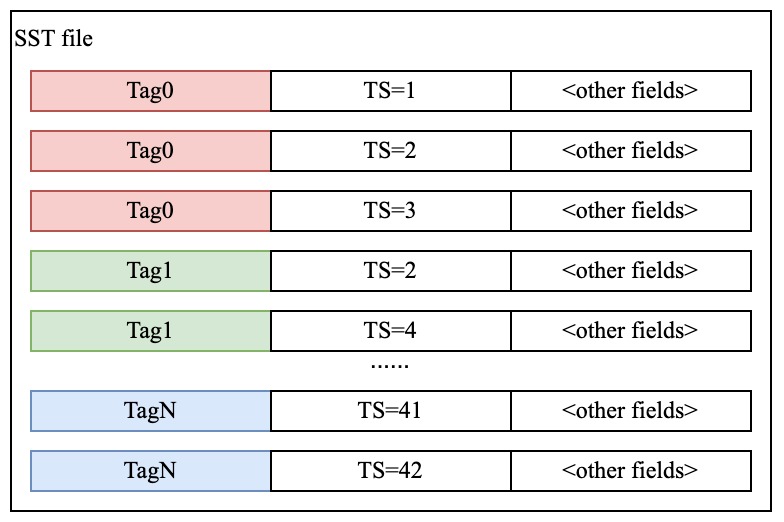
Typically, the time ranges of SST files do not overlap during real-time writing workloads. However, due to factors like row deletions and out-of-order writes, SST files may have overlapping time ranges, which can affect query performance.
### Time window
Time-series workloads present prominent "windowed" pattern in that most recently inserted rows are more possible to be read. Thus GreptimeDB logically partitioned the time axis into different time windows and we are more interested in compacting those SST files fall into the same time window.
Time window for some specific table is usually inferred from the most-recently flushed SST files or users may manually specify the time window if TWCS is chosen.
GreptimeDB has a preset collection of window sizes that are:
- 1 hour
- 2 hours
- 12 hours
- 1 day
- 1 week
If time window is not specified, GreptimeDB will use `1hour` as the initial time window size and split all inserted rows to those time windows and will infer a proper time window size when the first compaction happens by selecting the minimum time window size for the above collection that can cover the whole time span of all files to be compacted.
For example, during the first compaction, the time span for all SST files is 4 hours, then GreptimeDB will choose 12 hours as the time window for that table and persist it for later compactions.
### Sorted runs
Sorted runs is a collection of SST files that have sorted and non-overlapping time ranges.
For example, a table contains 5 SSTs with following time ranges (all inclusive): `[0, 10]`, `[12, 23]`, `[22, 25]`,`[24, 30]`,`[26,33]` and we can find 2 sorted runs:
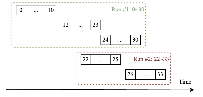
The number of sorted runs indicates the orderliness of SST files. More sorted runs typically lead to worse query performance. The main goal of compactions is to reduce the number of sorted runs.
### Levels
Databases based on LSM trees may also have levels, keys are merged level by level. GreptimeDB only has 2 levels which are 0 (uncompacted) and 1 (compacted).
## Compaction strategies
GreptimeDB provides two compaction strategies as mentioned above, but only Time Windowed Compaction Strategy (TWCS) can be chosen when creating tables. Strict Window Compaction Strategy (SWCS) is only available when executing manual compactions.
## Time Windowed Compaction Strategy (TWCS)
TWCS primarily aims to reduce read/write amplification during compaction.
It assigns files to be compacted into different time windows. For each window, TWCS identifies the sorted runs. If there are more than 1 sorted runs, TWCS finds a solution to merge the overlapping files in those runs with merging penalties taken into consideration. If there's only 1 sorted run, TWCS checks for excessive file fragmentation and merges fragmented files if necessary since SST file count also impacts query performance.
For window assignment, SST files may span multiple time windows. TWCS assigns SSTs based on their maximum timestamps to ensure they are not affected by stale data. In time-series workloads, out-of-order writes are infrequent, and even when they occur, recent data's query performance is more critical than that of stale data.
Common TWCS table options include:
- `trigger_file_num`: number of files in a specific time window to trigger a compaction (default 4).
- `time_window`: time window size for TWCS compaction.
- `max_output_file_size`: max allowed compaction output file size (default 512MB).
Following diagrams show how files in a window get compacted when `trigger_file_num = 3`:
- In A, there're two SST files `[0, 3]` and `[5, 6, 9]` but there's only one sorted run since those two files have disjoint time ranges.
- In B, a new SST file `[1, 4]` is flushed therefore forms two sorted runs that exceeds the threshold. Then `[0, 3]` and `[1, 4]` are merged to `[0, 1, 3, 4]`.
- In C, a new SST file `[9, 10]` is flushed, and it will be merged with `[5, 6, 10]` to create `[5, 6, 9, 10]`, and after compaction the files will be like D.
- In E, a new file `[11, 12]` is flushed. Though there's still only one sorted run, but the number of files reaches `trigger_file_num`(3), so `[5, 6, 9, 10]` will be merged with `[11, 12]` to form `[5, 6, 9, 10, 11, 12]`.
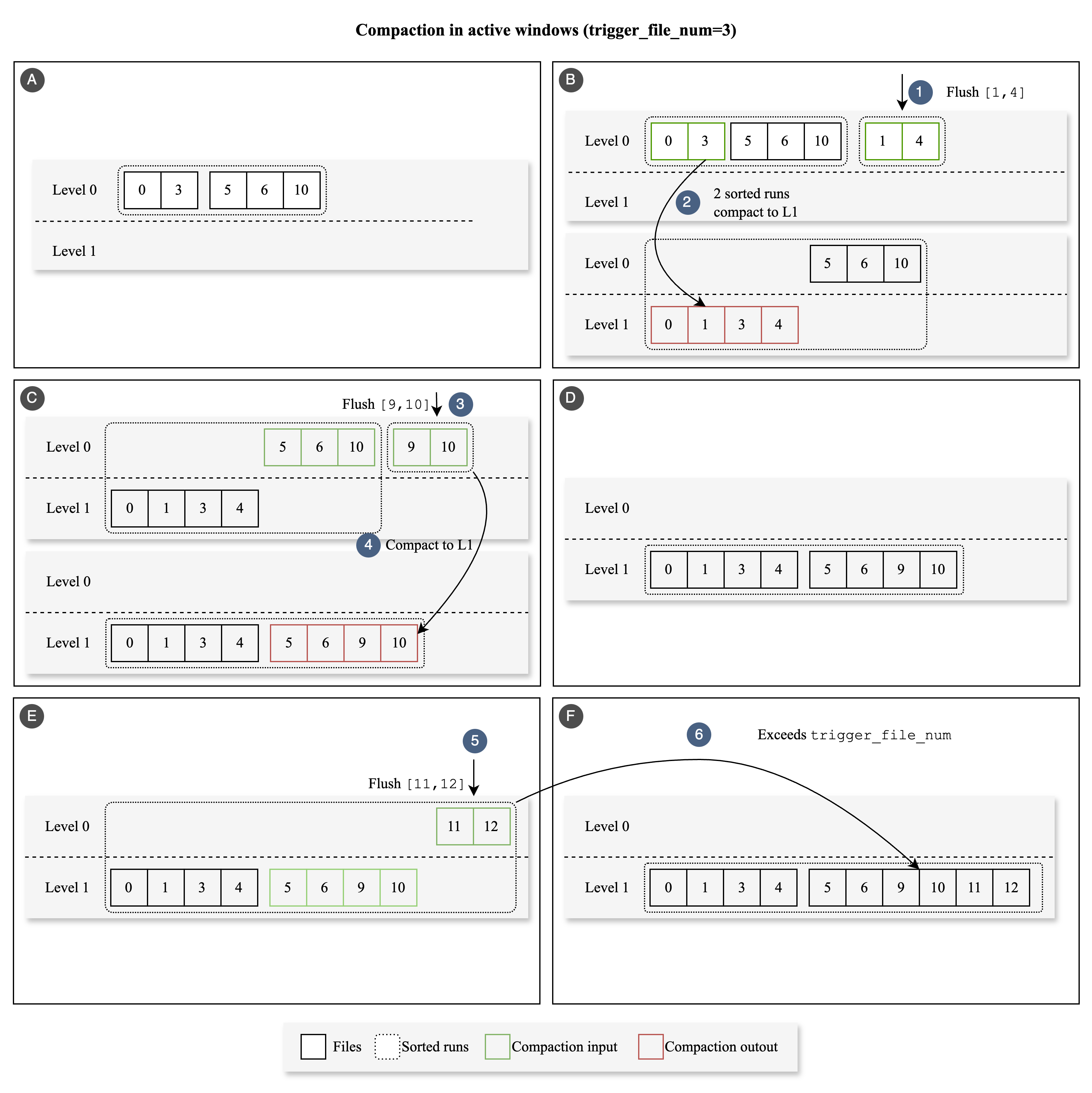
### Specifying TWCS parameters
TWCS parameters can be specified at two levels:
1. **Table level**: Explicitly set when creating or altering a table
2. **Database level**: Set as defaults for all tables in the database
The effective compaction settings are resolved dynamically at compaction scheduling time with the following priority:
- Table-level settings (if specified)
- Database-level settings (if specified and no table-level override)
- Built-in defaults
#### Table-level compaction settings
You can specify TWCS parameters when creating tables:
```sql
CREATE TABLE monitor (
host STRING,
ts TIMESTAMP DEFAULT CURRENT_TIMESTAMP() TIME INDEX,
cpu FLOAT64 DEFAULT 0,
memory FLOAT64,
PRIMARY KEY(host))
WITH (
'compaction.type'='twcs',
'compaction.twcs.trigger_file_num'='8',
'compaction.twcs.time_window'='1h',
'compaction.twcs.max_output_file_size'='500MB'
);
```
#### Database-level compaction settings
You can also set default compaction parameters for all tables in a database. These settings will be inherited by tables that don't have explicit compaction settings. See [ALTER DATABASE](/reference/sql/alter.md#modify-compaction-options-of-database) for examples.
:::note
Unlike table-level settings which are stored with the table metadata, database-level compaction settings are dynamically resolved at runtime. Changing database-level compaction options will immediately affect all tables in the database that don't have their own explicit compaction settings. This behavior is similar to how [database-level TTL](/reference/sql/create.md#create-database) works.
:::
## Strict Window Compaction Strategy (SWCS) and manual compaction
Unlike TWCS, which assigns one window per SST file based on their maximum timestamps, SWCS assigns SST files to **all** overlapping windows. Consequently, a single SST file may be included in multiple compaction outputs, as its name suggests. Due to its high read amplification during compaction, SWCS is not the default compaction strategy. However, it is useful when you need to manually trigger compaction to reorganize the layout of SST files—especially if an individual SST file spans a large time range that significantly slows down queries. GreptimeDB offers a simple SQL function for triggering compaction:
```sql
ADMIN COMPACT_TABLE(
,
,
[]
);
```
The `` parameter can be `regular` (or `twcs`) for regular TWCS compaction, or `swcs` (or `strict_window`) for Strict Window Compaction Strategy. The value is case-insensitive.
For the `swcs` strategy, the `` can specify:
- The window size (in seconds) for splitting SST files
- The `parallelism` parameter to control the level of parallelism for compaction (defaults to 1)
For example, to trigger compaction with a 1-hour window:
```sql
ADMIN COMPACT_TABLE(
"monitor",
"swcs",
"3600"
);
+------------------------------------------------+
| ADMIN COMPACT_TABLE("monitor", "swcs", "3600") |
+------------------------------------------------+
| 0 |
+------------------------------------------------+
1 row in set (0.01 sec)
```
When executing this statement, GreptimeDB will split each SST file into segments with a time span of 1 hour (3600 seconds) and merge these segments into a single output, ensuring no overlapping files remain.
You can also specify the `parallelism` parameter to speed up compaction by processing multiple files concurrently:
```sql
-- SWCS compaction with default time window and parallelism set to 2
ADMIN COMPACT_TABLE("monitor", "swcs", "parallelism=2");
-- SWCS compaction with custom time window and parallelism
ADMIN COMPACT_TABLE("monitor", "swcs", "window=1800,parallelism=2");
```
The `parallelism` parameter is also available for regular compaction:
```sql
-- Regular compaction with parallelism set to 2
ADMIN COMPACT_TABLE("monitor", "regular", "parallelism=2");
```
The following diagram shows the process of strict window compression:
In Figure A, there are 3 overlapping SST files: `[0, 3]` (which includes timestamps 0, 1, 2, and 3), `[3, 8]`, and `[8, 10]`.
The strict window compaction strategy will assign the file `[3, 8]` that covers windows 0, 4, and 8 to three separate windows respectively. This allows it to merge with `[0, 3]` and `[8, 10]` separately.
Figure B shows the final compaction result with three files: `[0, 3]`, `[4, 7]`, and `[8, 10]`. These files do not overlap with each other.
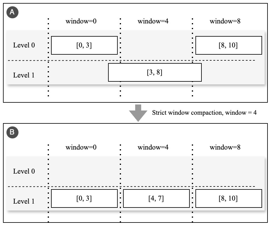
---
## Garbage Collection (GC)
GreptimeDB GC delays physical deletion of SST/index files until all references (running queries, [repartition](./repartition.md) cross-region file refs) are released. The configuration contains two parts:
- Metasrv Configuration
- Datanode Configuration
## How it works
- **Roles**: Meta decides when/where to clean; datanodes perform the actual delete while keeping in-use files safe.
- **Safety windows**: `lingering_time` holds known-removed files a bit longer; `unknown_file_lingering_time` is a rare-case guard.
- **Listing modes**: Fast mode removes files the system already marked; full listing walks storage to catch stragglers/orphans.

## Metasrv Configuration
On the Metasrv side, GC schedules cleanup tasks for regions and coordinates when to run GC.
```toml
[gc]
enable = true # Enable meta GC scheduler. default to be false; must match datanode.
gc_cooldown_period = "5m" # Minimum gap before the same region is GCed again.
```
### Options
| Configuration Option | Description |
| --- | --- |
| `enable` | Enable the meta GC scheduler. Must match datanode GC enablement. |
| `gc_cooldown_period` | Minimum interval before the same region is scheduled for GC again; keep datanode `lingering_time` longer than this. |
## Datanode Configuration
The Datanode side performs the actual deletion while protecting files still in use.
```toml
[[region_engine]]
[region_engine.mito]
[region_engine.mito.gc]
enable = true # Turn on datanode GC worker; must match meta.
lingering_time = "10m" # Keep known-removed files this long for active queries.
unknown_file_lingering_time = "1h" # Keep files without expel time; rare safeguard.
```
### Options
| Configuration Option | Description |
| --- | --- |
| `enable` | Enable the datanode GC worker. Must match meta GC `enable`. |
| `lingering_time` | How long to keep manifest-removed files before deletion to protect long follower-region queries/cross-region references; set longer than `gc_cooldown_period`. Use `"0s"` to delete immediately. |
| `unknown_file_lingering_time` | Safety hold for files without expel time (not tracked in manifest). Should be generous; these cases are rare. |
:::warning
`gc.enable` must be set consistently on metasrv and all datanodes. Mismatched flags cause GC to be skipped or stuck.
:::
## When to enable
- GC only applies when tables use object storage; tables on local filesystems ignore GC settings.
- Turn on GC if need to repartition so cross-region references can drain safely before deletion.
- For clusters with long-running follower-region queries, turn on GC and set `lingering_time` longer than `gc_cooldown_period` so files created or referenced during a GC cycle stay alive (in-use or lingering) until at least the next cycle.
- Leave GC off if you are not repartitioning and do not need delayed deletion.
## Operational notes
- GC is designed for object storage backends (with list/delete support); ensure your store credentials and permissions allow listing and deletion.
- Deleted files live in object storage until GC removes them; ensure storage listing/deletion permissions are in place.
- After enabling, restart metasrv and datanodes to apply config changes.
---
## Manage Data
---
## Region Failover
Region Failover provides the ability to recover regions from region failures. With Kafka WAL (Remote WAL) and shared storage, Region Failover can recover regions without losing data. This is implemented via [Region Migration](/user-guide/deployments-administration/manage-data/region-migration.md).
## Enable the Region Failover
This feature is only available on GreptimeDB running on distributed mode and
- Using Kafka WAL (Remote WAL) or Local WAL with `allow_region_failover_on_local_wal=true` (enabling region failover on Local WAL may lead to data loss during failover)
- Using [shared storage](/user-guide/deployments-administration/configuration.md#storage-options) (e.g., AWS S3)
If you want to enable region failover on local WAL, you need to set `allow_region_failover_on_local_wal=true` in [metasrv](/user-guide/deployments-administration/configuration.md#metasrv-only-configuration) configuration file. It's not recommended to enable this option, because it may lead to data loss.
### Via configuration file
Set `enable_region_failover=true` in the [metasrv](/user-guide/deployments-administration/configuration.md#metasrv-only-configuration) configuration file. Additionally, set `region_failure_detector_initialization_delay` to a larger value and enable [Cluster Maintenance Mode](/user-guide/deployments-administration/maintenance/maintenance-mode.md) within the `region_failure_detector_initialization_delay` period to avoid triggering unnecessary Region Failover during datanode startup or upgrades.
### Via GreptimeDB Operator
To enable region failover via GreptimeDB Operator, you can refer to [Common Helm Chart Configurations](/user-guide/deployments-administration/deploy-on-kubernetes/common-helm-chart-configurations.md#enable-region-failover) for more details.
## The recovery time of Region Failover
The recovery time of Region Failover with Kafka WAL (Remote WAL) depends on:
- number of regions per Topic.
- the Kafka cluster read throughput performance.
### The read amplification
In best practices, [the number of topics/partitions supported by a Kafka cluster is limited](https://docs.aws.amazon.com/msk/latest/developerguide/bestpractices.html) (exceeding this number can degrade Kafka cluster performance).
Therefore, we allow multiple regions to share a single topic as the WAL.
However, this may cause to the read amplification issue.
The data belonging to a specific region consists of data files plus data in the WAL (typically `WAL[LastCheckpoint...Latest]`). The failover of a specific region only requires reading the region's WAL data to reconstruct the memory state, which is called region replaying. However, If multiple regions share a single topic, replaying data for a specific region from the topic requires filtering out unrelated data (i.e., data from other regions). This means replaying data for a specific region from the topic requires reading more data than the actual size of the region's data in the topic, a phenomenon known as read amplification.
Although multiple regions share the same topic, allowing the Datanode to support more regions, the cost of this approach is read amplification during WAL replay.
For example, configure 128 topics for [metasrv](/user-guide/deployments-administration/configuration.md#metasrv-only-configuration), and if the whole cluster holds 1024 regions (physical regions), every 8 regions will share one topic.
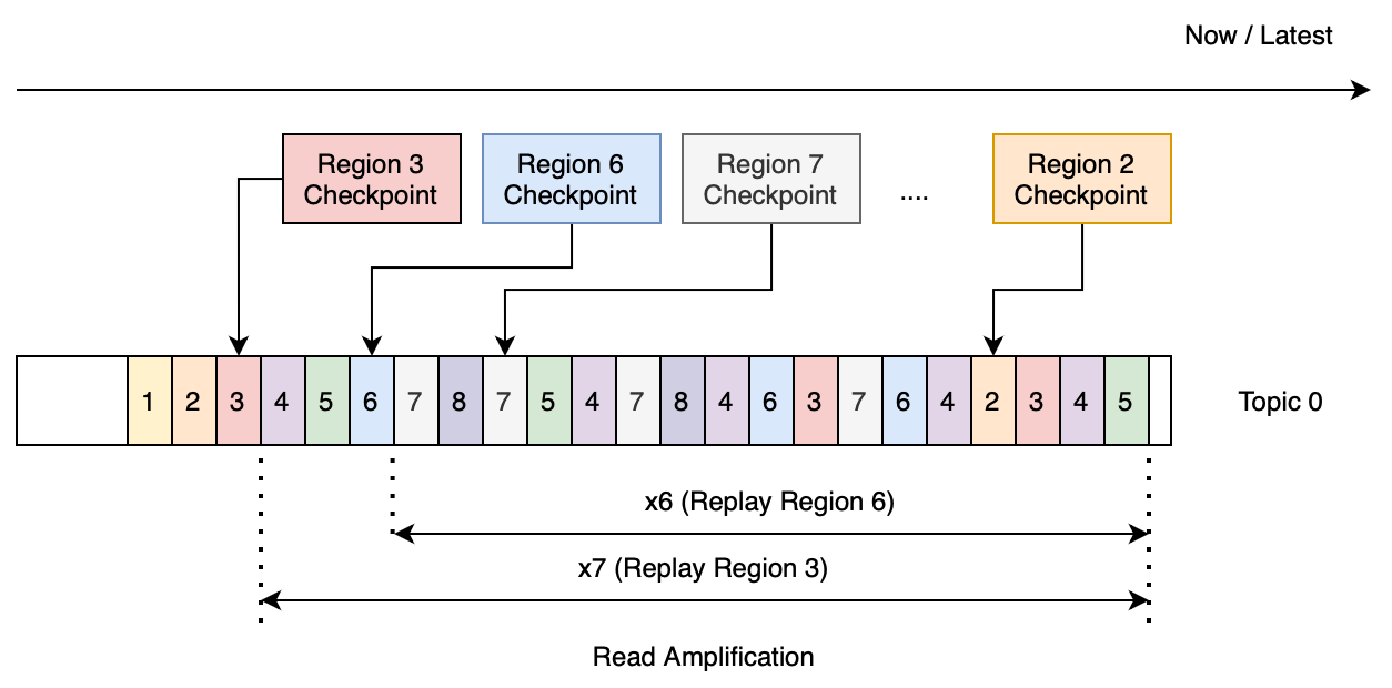
(Figure1: recovery Region 3 need to read redundant data 7 times larger than the actual size)
A simple model to estimate the redundant read amplification factor (redundant replay data size/actual data size):
- For a single topic, if we try to replay all regions that belong to the topic, then the amplification factor would be 7+6+...+1 = 28 times. (The Region WAL data distribution is shown in the Figure 1. Replaying Region 3 will read 7 times redundant data larger than the actual size; Region 6 will read 6 times, and so on)
- When recovering 100 regions (requiring about 13 topics), the amplification factor is approximately 28 \* 13 = 364 times.
Assuming we have 100 regions to recover, and the actual data size of all regions is 0.5GB, the following table shows the replay data size based on the number of regions per topic.
| Number of regions per Topic | Number of topics required for 100 Regions | Single topic redundant read factor | Total redundant read factor | Replay data size (GB) |
| --------------------------- | ----------------------------------------- | -------------------------------------- | ---------------------------------- | ---------------- |
| 1 | 100 | 0 | 0 | 0.5 |
| 2 | 50 | 1 | 50 | 25.5 |
| 4 | 25 | 6 | 150 | 75.5 |
| 8 | 13 | 28 | 364 | 182.5 |
| 16 | 7 | 120 | 840 | 420.5 |
The following table shows the recovery time of 100 regions under different read throughput conditions of the Kafka cluster. For example, when providing a read throughput of 300MB/s, recovering 100 regions requires approximately 10 minutes (182.5GB/0.3GB = 10m).
| Number of regions per Topic | Replay data size (GB) | Kafka throughput 300MB/s- Recovery time (secs) | Kafka throughput 1000MB/s- Recovery time (secs) |
| --------------------------- | ---------------- | --------------------------------------------- | ---------------------------------------------- |
| 1 | 0.5 | 2 | 1 |
| 2 | 25.5 | 85 | 26 |
| 4 | 75.5 | 252 | 76 |
| 8 | 182.5 | 608 | 183 |
| 16 | 420.5 | 1402 | 421 |
### Suggestions for improving recovery time
In the above example, we calculated the recovery time based on the number of Regions contained in each Topic for reference.
We have calculated the recovery time under different Number of regions per Topic configuration for reference.
In actual scenarios, the read amplification may be larger than this model.
If you use Kafka WAL and are very sensitive to recovery time, we recommend that each region have its own topic (i.e., Number of regions per Topic is 1).
---
## Region Migration
Region Migration allows users to move regions between the Datanode.
:::warning Warning
This feature is only available on GreptimeDB running on distributed mode and
- Using [shared storage](/user-guide/deployments-administration/configuration.md#storage-options) (e.g., AWS S3)
Otherwise, you can't perform a region migration.
:::
## Figure out the region distribution of the table.
You need to first query the region distribution of the table, i.e., find out on which Datanode the Regions in the table are located.
```sql
select b.peer_id as datanode_id,
a.greptime_partition_id as region_id
from information_schema.partitions a left join information_schema.region_peers b
on a.greptime_partition_id = b.region_id where a.table_name='migration_target' order by datanode_id asc;
```
For example, have the following region distribution:
```sql
+-------------+---------------+
| datanode_id | region_id |
+-------------+---------------+
| 1 | 4398046511104 |
+-------------+---------------+
1 row in set (0.01 sec)
```
For more info about the `region_peers` table, please read the [REGION-PEERS](/reference/sql/information-schema/region-peers.md).
## Select a Datanode as the migration destination.
:::warning Warning
The region migration won't be performed if the `from_peer_id` equals the `to_peer_id`.
:::
Remember, if you deploy the cluster via the GreptimeDB operator, the `peer_id` of Datanode always starts from 0. For example, if you have a 3 Datanode GreptimeDB cluster, the available `peer_id` will be 0,1,2.
Finally, you can do a Region migration request via the following SQL:
```sql
ADMIN migrate_region(4398046511104, 1, 2, 60);
```
The parameters of `migrate_region`:
```sql
ADMIN migrate_region(region_id, from_peer_id, to_peer_id);
ADMIN migrate_region(region_id, from_peer_id, to_peer_id, replay_timeout);
```
| Option | Description | Required | |
| ---------------- | ----------------------------------------------------------------------------------------------------------------------------------------------------------------------------------------- | ------------ | --- |
| `region_id` | The region id. | **Required** | |
| `from_peer_id` | The peer id of the migration source(Datanode). | **Required** | |
| `to_peer_id` | The peer id of the migration destination(Datanode). | **Required** | |
| `replay_timeout` | The timeout (in seconds) for replaying data. Defaults to 300 seconds if omitted. If the new Region fails to replay the data within the specified timeout, the migration will fail, however the data in the old Region will not be lost. | Optional | |
## Query the migration state
The `migrate_region` function returns the procedure id that executes the migration, queries the procedure state by it:
```sql
ADMIN procedure_state('538b7476-9f79-4e50-aa9c-b1de90710839')
```
If it's done, outputs the state in JSON:
```json
{"status":"Done"}
```
Of course, you can confirm the region distribution by querying from `region_peers` and `partitions` in `information_schema`.
---
## Repartition
Repartition lets you adjust partition rules after a table has been created.
GreptimeDB does this through `ALTER TABLE` partition split and merge operations; see [ALTER TABLE](/reference/sql/alter.md#split-or-merge-partitions) for the syntax.
Repartition is only supported in distributed clusters.
## How it works
The core idea is to adjust partition rules and Region routing online instead of manually moving data into a new table.
GreptimeDB switches to the new partition layout by updating manifest file references for each Region, so the rules can better match the current data distribution.
This approach is useful when traffic patterns change over time and you want to keep partition rules aligned with the workload without rebuilding the table.
During repartitioning, writes may be briefly affected, so client-side retries are recommended.
## When to repartition
Consider repartitioning when:
- Some regions are consistently hotter than others.
- Your data distribution changes and the current partition boundaries no longer fit.
- Some regions become very small and cold, and you want to reduce resource usage by merging them.
- You want to further split a partition to improve write concurrency or query performance.
In general, when partition rules no longer reflect the current data distribution well, it is worth considering repartitioning.
## How to identify hot partitions
Before repartitioning, confirm which regions are hot.
Join region statistics with partition metadata to find the hottest rules:
```sql
SELECT
t.table_name,
r.region_id,
r.region_number,
p.partition_name,
p.partition_description,
r.region_role,
r.written_bytes_since_open,
r.region_rows
FROM information_schema.region_statistics r
JOIN information_schema.tables t
ON r.table_id = t.table_id
JOIN information_schema.partitions p
ON p.table_schema = t.table_schema
AND p.table_name = t.table_name
AND p.greptime_partition_id = r.region_id
WHERE t.table_schema = 'public'
AND t.table_name = 'your_table'
ORDER BY r.written_bytes_since_open DESC
LIMIT 10;
```
If some regions have a much higher `written_bytes_since_open` value over time, that partition rule is usually a good candidate for splitting.
Also check whether the region peers are healthy so node issues are not mistaken for hotspots:
```sql
SELECT
p.region_id,
p.peer_addr,
p.status,
p.down_seconds
FROM information_schema.region_peers p
WHERE p.table_schema = 'public'
AND p.table_name = 'your_table'
ORDER BY p.region_id, p.peer_addr;
```
If the nodes are healthy and the hotspot signal persists, you can move on to designing the repartition plan.
## Prerequisites
:::warning Warning
This feature is only available in distributed clusters and requires:
- Using [shared object storage](/user-guide/deployments-administration/configuration.md#storage-options) (e.g., AWS S3)
- Using [GC](/user-guide/deployments-administration/manage-data/gc.md) on both metasrv and all datanodes
Otherwise, you can't perform repartitioning.
:::
GreptimeDB supports repartitioning through repeated `SPLIT PARTITION` and `MERGE PARTITION` operations.
The most common cases are 1-to-2 splits and 2-to-1 merges.
More complex changes can also be done step by step.
Object storage stores region files, while GC reclaims old files only after references are released.
This helps prevent accidental deletion of data still in use.
### Through GreptimeDB Operator
If you deploy GreptimeDB with the GreptimeDB Operator, refer to [Common Helm Chart Configurations](/user-guide/deployments-administration/deploy-on-kubernetes/common-helm-chart-configurations.md) for GC and object storage setup.
## Example
You can repartition a table by merging existing partitions and then splitting them with new rules.
The following example changes the `area` partition key from `South` to `North` for devices with `device_id < 100`:
```sql
ALTER TABLE sensor_readings MERGE PARTITION (
device_id < 100 AND area < 'South',
device_id < 100 AND area >= 'South'
);
ALTER TABLE sensor_readings SPLIT PARTITION (
device_id < 100
) INTO (
device_id < 100 AND area < 'North',
device_id < 100 AND area >= 'North'
);
```
## Further reading
For a step-by-step tutorial with more background and examples, see [How to Split and Merge Partitions Online in GreptimeDB](https://greptime.com/blogs/2026-03-19-greptimedb-repartition-guide).
---
## Table Sharding
Table sharding is a technique used to distribute a large table into multiple smaller tables.
This practice is commonly employed to enhance the performance of database systems.
In GreptimeDB, data is logically sharded into partitions.
Since GreptimeDB uses "tables" to group data and SQL to query them,
we adopt the term "partition," a concept frequently used in OLTP databases.
## When to shard a table
Inside GreptimeDB, both data management and scheduling are based on the region level,
and each region is corresponding to a table partition.
Thus when you have a table that is too large to fit into a single node,
or the table is too hot to be served by a single node,
you should consider sharding it.
A region in GreptimeDB has a relative fixed throughput capacity,
and the number of regions in a table determines the total throughput capacity of the table.
If you want to increase the throughput capacity of a table,
you can increase the number of regions in the table.
Ideally the overall throughput of a table should be proportional to the number of regions.
As for which specific partition column to use or how many regions to create,
it depends on the data distribution and the query pattern.
A general goal is to make the data distribution among regions as even as possible.
And the query pattern should be considered when designing the partition rule set as one query can be processed in parallel among regions.
In other word the query latency is depends on the "slowest" region's latency.
But notice that the increase of regions will bring some basic consumption and increase the complexity of the system.
You need to consider the requirement of data ingest rate, the query performance,
the data distribution on storage system.
You should shard a table only when necessary.
For more information on the relationship between partitions and regions, refer to the [Table Sharding](/contributor-guide/frontend/table-sharding.md) section in the contributor guide.
## Partition
In GreptimeDB, a table can be horizontally partitioned by column value ranges.
Currently, GreptimeDB supports range partitioning with the `PARTITION ON COLUMNS` syntax.
Each partition includes only a portion of the data from the table, and is
grouped by some column(s) value range. For example, we can partition a table in GreptimeDB like
this:
```sql
CREATE TABLE (...)
PARTITION ON COLUMNS () (
);
```
The syntax mainly consists of two parts:
1. `PARTITION ON COLUMNS` followed by a comma-separated list of column names. This specifies which columns will be used for partitioning. The columns specified here must be of the Tag type (as specified by the PRIMARY KEY). Note that the ranges of all partitions must **not** overlap.
2. `RULE LIST` is a list of multiple partition rules. Each rule is a partition condition, and GreptimeDB generates partition names such as `p0`, `p1`, and so on for these rules. The expressions here can use `=`, `!=`, `>`, `>=`, `<`, `<=`, `AND`, `OR`, column names, and literals.
:::tip Note
The parentheses in `PARTITION ON COLUMNS (...)` only accept column names (e.g., `device_id`, `area`), not expressions like `device_id + 1`. GreptimeDB does not support MySQL's `PARTITION BY RANGE` syntax.
:::
### Example
## Create a distributed table
You can use the MySQL CLI to [connect to GreptimeDB](/user-guide/protocols/mysql.md) and create a distributed table.
The following example creates a table and partitions it based on the `device_id` column.
```SQL
CREATE TABLE sensor_readings (
device_id INT16,
reading_value FLOAT64,
ts TIMESTAMP DEFAULT current_timestamp(),
PRIMARY KEY (device_id),
TIME INDEX (ts)
)
PARTITION ON COLUMNS (device_id) (
device_id < 100,
device_id >= 100 AND device_id < 200,
device_id >= 200
);
```
More partition columns can be used to create more complex partition rules:
```sql
CREATE TABLE sensor_readings (
device_id INT,
area STRING,
reading_value FLOAT64,
ts TIMESTAMP DEFAULT current_timestamp(),
PRIMARY KEY (device_id, area),
TIME INDEX (ts)
)
PARTITION ON COLUMNS (device_id, area) (
device_id < 100 AND area < 'South',
device_id < 100 AND area >= 'South',
device_id >= 100 AND area <= 'East',
device_id >= 100 AND area > 'East'
);
```
The following content uses the `sensor_readings` table with two partition columns as an example.
## Repartition a sharded table
If you need to modify partition rules for an existing table, refer to the separate [Repartition](/user-guide/deployments-administration/manage-data/repartition.md) page.
## Insert data into the table
The following code inserts 3 rows into each partition of the `sensor_readings` table.
```sql
INSERT INTO sensor_readings (device_id, area, reading_value, ts)
VALUES (1, 'North', 22.5, '2023-09-19 08:30:00'),
(10, 'North', 21.8, '2023-09-19 09:45:00'),
(50, 'North', 23.4, '2023-09-19 10:00:00');
INSERT INTO sensor_readings (device_id, area, reading_value, ts)
VALUES (20, 'South', 20.1, '2023-09-19 11:15:00'),
(40, 'South', 19.7, '2023-09-19 12:30:00'),
(90, 'South', 18.9, '2023-09-19 13:45:00');
INSERT INTO sensor_readings (device_id, area, reading_value, ts)
VALUES (110, 'East', 25.3, '2023-09-19 14:00:00'),
(120, 'East', 26.5, '2023-09-19 15:30:00'),
(130, 'East', 27.8, '2023-09-19 16:45:00');
INSERT INTO sensor_readings (device_id, area, reading_value, ts)
VALUES (150, 'West', 24.1, '2023-09-19 17:00:00'),
(170, 'West', 22.9, '2023-09-19 18:15:00'),
(180, 'West', 23.7, '2023-09-19 19:30:00');
```
:::tip NOTE
Note that when the written data does not meet any of the rules in the partitioning scheme, it will be assigned to the default partition (i.e., the first partition 0 of the table).
:::
## Distributed Read
Simply use the `SELECT` statement to query the data:
```sql
SELECT * FROM sensor_readings order by reading_value desc LIMIT 5;
```
```sql
+-----------+------+---------------+---------------------+
| device_id | area | reading_value | ts |
+-----------+------+---------------+---------------------+
| 130 | East | 27.8 | 2023-09-19 16:45:00 |
| 120 | East | 26.5 | 2023-09-19 15:30:00 |
| 110 | East | 25.3 | 2023-09-19 14:00:00 |
| 150 | West | 24.1 | 2023-09-19 17:00:00 |
| 180 | West | 23.7 | 2023-09-19 19:30:00 |
+-----------+------+---------------+---------------------+
5 rows in set (0.02 sec)
```
```sql
SELECT MAX(reading_value) AS max_reading
FROM sensor_readings;
```
```sql
+-------------+
| max_reading |
+-------------+
| 27.8 |
+-------------+
1 row in set (0.03 sec)
```
```sql
SELECT * FROM sensor_readings
WHERE area = 'North' AND device_id < 50
ORDER BY device_id;
```
```sql
+-----------+-------+---------------+---------------------+
| device_id | area | reading_value | ts |
+-----------+-------+---------------+---------------------+
| 1 | North | 22.5 | 2023-09-19 08:30:00 |
| 10 | North | 21.8 | 2023-09-19 09:45:00 |
+-----------+-------+---------------+---------------------+
2 rows in set (0.03 sec)
```
## Inspect a sharded table
GreptimeDB provides severals system table to check DB's state. For table sharding information, you can query [`information_schema.partitions`](/reference/sql/information-schema/partitions.md) which gives the detail of partitions inside one table, and [`information_schema.region_peers`](/reference/sql/information-schema/region-peers.md) which gives the runtime distribution of regions.
---
## Metadata Storage Configuration
This section describes how to configure different metadata storage backends for the GreptimeDB Metasrv component. The metadata storage is used to store critical system information including catalogs, schemas, tables, regions, and other metadata that are essential for the operation of GreptimeDB.
## Available Storage Backends
GreptimeDB supports the following metadata storage backends:
- **etcd**: The default and recommended backend for development and testing environments, offering simplicity and ease of setup
- **MySQL/PostgreSQL**: Production-ready backend options that integrate well with existing database infrastructure and cloud RDS services
This documentation describes the TOML configuration for each backend. You can use these configurations when deploying GreptimeDB without Helm Chart.
If you are using Helm Chart to deploy GreptimeDB, please refer to [Common Helm Chart Configurations](/user-guide/deployments-administration/deploy-on-kubernetes/common-helm-chart-configurations.md#configuring-metasrv-backend-storage) for more details.
## Use etcd as metadata storage
While etcd is suitable for development and testing environments, it may not be ideal for production deployments requiring high availability and scalability.
Configure the metasrv component to use etcd as metadata storage:
```toml
# The metadata storage backend for metasrv
backend = "etcd_store"
# Store server addresses
# You can specify multiple etcd endpoints for high availability
store_addrs = ["127.0.0.1:2379"]
# Backend client options for etcd
[backend_client]
# The keep alive timeout for backend client
keep_alive_timeout = "3s"
# The keep alive interval for backend client
keep_alive_interval = "10s"
# The connect timeout for backend client
connect_timeout = "3s"
[backend_tls]
# - "disable" - No TLS
# - "require" - Require TLS
mode = "prefer"
# Path to client certificate file (for client authentication)
# Like "/path/to/client.crt"
cert_path = ""
# Path to client private key file (for client authentication)
# Like "/path/to/client.key"
key_path = ""
# Path to CA certificate file (for server certificate verification)
# Required when using custom CAs or self-signed certificates
# Leave empty to use system root certificates only
# Like "/path/to/ca.crt"
ca_cert_path = ""
```
### Best Practices
While etcd can be used as metadata storage, we recommend against using it in production environments unless you have extensive experience with etcd operations and maintenance. For detailed guidance on etcd management, including installation, backup, and maintenance procedures, please refer to [Manage etcd](/user-guide/deployments-administration/manage-metadata/manage-etcd.md).
When using etcd as metadata storage:
- Deploy multiple endpoints across different availability zones for high availability
- Configure appropriate auto-compaction settings to manage storage growth
- Implement regular maintenance procedures:
- Run `Defrag` command periodically to reclaim disk space
- Monitor etcd cluster health metrics
- Review and adjust resource limits based on usage patterns
## Use MySQL as metadata storage
MySQL serves as a viable metadata storage backend option. This choice is particularly beneficial when you need to integrate with existing MySQL infrastructure or have specific MySQL-related requirements. For production deployments, we strongly recommend utilizing cloud providers' Relational Database Service (RDS) solutions for enhanced reliability and managed service benefits.
Configure the metasrv component to use MySQL as metadata storage:
```toml
# The metadata storage backend for metasrv
backend = "mysql_store"
# Store server address
# Format: mysql://user:password@ip:port/dbname
store_addrs = ["mysql://user:password@ip:port/dbname"]
# Optional: Custom table name for storing metadata
# Default: greptime_metakv
meta_table_name = "greptime_metakv"
[backend_tls]
# - "disable" - No TLS
# - "prefer" (default) - Try TLS, fallback to plain
# - "require" - Require TLS
# - "verify_ca" - Require TLS and verify CA
# - "verify_full" - Require TLS and verify hostname
mode = "prefer"
# Path to client certificate file (for client authentication)
# Like "/path/to/client.crt"
cert_path = ""
# Path to client private key file (for client authentication)
# Like "/path/to/client.key"
key_path = ""
# Path to CA certificate file (for server certificate verification)
# Required when using custom CAs or self-signed certificates
# Leave empty to use system root certificates only
# Like "/path/to/ca.crt"
ca_cert_path = ""
```
When sharing a MySQL instance between multiple GreptimeDB clusters, you must set a unique `meta_table_name` for each GreptimeDB cluster to avoid metadata conflicts.
## Use PostgreSQL as metadata storage
PostgreSQL serves as a viable metadata storage backend option. This choice is particularly beneficial when you need to integrate with existing PostgreSQL infrastructure or have specific PostgreSQL-related requirements. For production deployments, we strongly recommend utilizing cloud providers' Relational Database Service (RDS) solutions for enhanced reliability and managed service benefits.
Configure the metasrv component to use PostgreSQL as metadata storage:
```toml
# The metadata storage backend for metasrv
backend = "postgres_store"
# Store server address
# Format: password=password dbname=postgres user=postgres host=localhost port=5432
store_addrs = ["password=password dbname=postgres user=postgres host=localhost port=5432"]
# Optional: Custom table name for storing metadata
# Default: greptime_metakv
meta_table_name = "greptime_metakv"
# Optional: The schema for metadata table and election table name.
# In PostgreSQL 15 and later, the default public schema is restricted by default,
# and non-superusers are no longer allowed to create tables in the public schema.
# When encountering permission restrictions, use this parameter to specify a writable schema.
meta_schema_name = "greptime_schema"
# Optional: Automatically create PostgreSQL schema if it doesn't exist.
# When enabled, the system will execute `CREATE SCHEMA IF NOT EXISTS `
# before creating metadata tables. This is useful in production environments where
# manual schema creation may be restricted.
# Default: true
# Note: The PostgreSQL user must have CREATE SCHEMA permission for this to work.
auto_create_schema = true
# Optional: Advisory lock ID for election
# Default: 1
meta_election_lock_id = 1
[backend_tls]
# - "disable" - No TLS
# - "prefer" (default) - Try TLS, fallback to plain
# - "require" - Require TLS
# - "verify_ca" - Require TLS and verify CA
# - "verify_full" - Require TLS and verify hostname
mode = "prefer"
# Path to client certificate file (for client authentication)
# Like "/path/to/client.crt"
cert_path = ""
# Path to client private key file (for client authentication)
# Like "/path/to/client.key"
key_path = ""
# Path to CA certificate file (for server certificate verification)
# Required when using custom CAs or self-signed certificates
# Leave empty to use system root certificates only
# Like "/path/to/ca.crt"
ca_cert_path = ""
```
When sharing a PostgreSQL instance between multiple GreptimeDB clusters or with other applications, you must configure two unique identifiers to prevent conflicts:
1. Set a unique `meta_table_name` for each GreptimeDB cluster to avoid metadata conflicts
2. Assign a unique `meta_election_lock_id` to each GreptimeDB cluster to prevent advisory lock conflicts with other applications using the same PostgreSQL instance
---
## Manage etcd
The GreptimeDB cluster requires an etcd cluster for [metadata storage](https://docs.greptime.com/nightly/contributor-guide/metasrv/overview) by default. Let's install an etcd cluster using Bitnami's etcd Helm [chart](https://github.com/bitnami/charts/tree/main/bitnami/etcd).
## Prerequisites
- [Kubernetes](https://kubernetes.io/docs/setup/) >= v1.23
- [kubectl](https://kubernetes.io/docs/tasks/tools/install-kubectl/) >= v1.18.0
- [Helm](https://helm.sh/docs/intro/install/) >= v3.0.0
## Install
Save the following configuration as a file `etcd.yaml`:
```yaml
global:
security:
allowInsecureImages: true
replicaCount: 3
image:
registry: docker.io
repository: greptime/etcd
tag: 3.6.1-debian-12-r3
auth:
rbac:
create: false
token:
enabled: false
persistence:
storageClass: null
size: 8Gi
resources:
limits:
cpu: '2'
memory: 8Gi
requests:
cpu: '2'
memory: 8Gi
autoCompactionMode: "periodic"
autoCompactionRetention: "1h"
extraEnvVars:
- name: ETCD_QUOTA_BACKEND_BYTES
value: "8589934592"
- name: ETCD_ELECTION_TIMEOUT
value: "2000"
- name: ETCD_SNAPSHOT_COUNT
value: "10000"
```
Install etcd cluster:
```bash
helm upgrade --install etcd \
oci://registry-1.docker.io/bitnamicharts/etcd \
--create-namespace \
--version 12.0.8 \
-n etcd-cluster \
--values etcd.yaml
```
Wait for etcd cluster to be running:
```bash
kubectl get pod -n etcd-cluster
```
Expected Output
```bash
NAME READY STATUS RESTARTS AGE
etcd-0 1/1 Running 0 64s
etcd-1 1/1 Running 0 65s
etcd-2 1/1 Running 0 72s
```
When the etcd cluster is running, use the following command to check the health status of etcd cluster:
```bash
kubectl -n etcd-cluster \
exec etcd-0 -- etcdctl \
--endpoints etcd-0.etcd-headless.etcd-cluster:2379,etcd-1.etcd-headless.etcd-cluster:2379,etcd-2.etcd-headless.etcd-cluster:2379 \
endpoint status -w table
```
Expected Output
```bash
+----------------------------------------+------------------+---------+---------+-----------+------------+-----------+------------+--------------------+--------+
| ENDPOINT | ID | VERSION | DB SIZE | IS LEADER | IS LEARNER | RAFT TERM | RAFT INDEX | RAFT APPLIED INDEX | ERRORS |
+----------------------------------------+------------------+---------+---------+-----------+------------+-----------+------------+--------------------+--------+
| etcd-0.etcd-headless.etcd-cluster:2379 | 680910587385ae31 | 3.5.15 | 20 kB | false | false | 4 | 73991 | 73991 | |
| etcd-1.etcd-headless.etcd-cluster:2379 | d6980d56f5e3d817 | 3.5.15 | 20 kB | false | false | 4 | 73991 | 73991 | |
| etcd-2.etcd-headless.etcd-cluster:2379 | 12664fc67659db0a | 3.5.15 | 20 kB | true | false | 4 | 73991 | 73991 | |
+----------------------------------------+------------------+---------+---------+-----------+------------+-----------+------------+--------------------+--------+
```
## Backup
In the bitnami etcd chart, a shared storage volume Network File System (NFS) is used to store etcd backup data. By using CronJob in Kubernetes to perform etcd snapshot backups and mount NFS PersistentVolumeClaim (PVC), snapshots can be transferred to NFS.
Add the following configuration and name it `etcd-backup.yaml` file, Note that you need to modify **existingClaim** to your NFS PVC name:
```yaml
global:
security:
allowInsecureImages: true
replicaCount: 3
image:
registry: docker.io
repository: greptime/etcd
tag: 3.6.1-debian-12-r3
auth:
rbac:
create: false
token:
enabled: false
persistence:
storageClass: null
size: 8Gi
resources:
limits:
cpu: '2'
memory: 8Gi
requests:
cpu: '2'
memory: 8Gi
autoCompactionMode: "periodic"
autoCompactionRetention: "1h"
extraEnvVars:
- name: ETCD_QUOTA_BACKEND_BYTES
value: "8589934592"
- name: ETCD_ELECTION_TIMEOUT
value: "2000"
- name: ETCD_SNAPSHOT_COUNT
value: "10000"
# Backup settings
disasterRecovery:
enabled: true
cronjob:
schedule: "*/30 * * * *"
historyLimit: 2
snapshotHistoryLimit: 2
pvc:
existingClaim: "${YOUR_NFS_PVC_NAME_HERE}"
```
Redeploy etcd cluster:
```bash
helm upgrade --install etcd \
oci://registry-1.docker.io/bitnamicharts/etcd \
--create-namespace \
--version 12.0.8 \
-n etcd-cluster \
--values etcd-backup.yaml
```
You can see the etcd backup scheduled task:
```bash
kubectl get cronjob -n etcd-cluster
```
Expected Output
```bash
NAME SCHEDULE TIMEZONE SUSPEND ACTIVE LAST SCHEDULE AGE
etcd-snapshotter */30 * * * * False 0 36s
```
```bash
kubectl get pod -n etcd-cluster
```
Expected Output
```bash
NAME READY STATUS RESTARTS AGE
etcd-0 1/1 Running 0 35m
etcd-1 1/1 Running 0 36m
etcd-2 0/1 Running 0 6m28s
etcd-snapshotter-28936038-tsck8 0/1 Completed 0 4m49s
```
```bash
kubectl logs etcd-snapshotter-28936038-tsck8 -n etcd-cluster
```
Expected Output
```log
etcd-0.etcd-headless.etcd-cluster.svc.cluster.local:2379 is healthy: successfully committed proposal: took = 2.698457ms
etcd 11:18:07.47 INFO ==> Snapshotting the keyspace
{"level":"info","ts":"2025-01-06T11:18:07.579095Z","caller":"snapshot/v3_snapshot.go:65","msg":"created temporary db file","path":"/snapshots/db-2025-01-06_11-18.part"}
{"level":"info","ts":"2025-01-06T11:18:07.580335Z","logger":"client","caller":"v3@v3.5.15/maintenance.go:212","msg":"opened snapshot stream; downloading"}
{"level":"info","ts":"2025-01-06T11:18:07.580359Z","caller":"snapshot/v3_snapshot.go:73","msg":"fetching snapshot","endpoint":"etcd-0.etcd-headless.etcd-cluster.svc.cluster.local:2379"}
{"level":"info","ts":"2025-01-06T11:18:07.582124Z","logger":"client","caller":"v3@v3.5.15/maintenance.go:220","msg":"completed snapshot read; closing"}
{"level":"info","ts":"2025-01-06T11:18:07.582688Z","caller":"snapshot/v3_snapshot.go:88","msg":"fetched snapshot","endpoint":"etcd-0.etcd-headless.etcd-cluster.svc.cluster.local:2379","size":"20 kB","took":"now"}
{"level":"info","ts":"2025-01-06T11:18:07.583008Z","caller":"snapshot/v3_snapshot.go:97","msg":"saved","path":"/snapshots/db-2025-01-06_11-18"}
Snapshot saved at /snapshots/db-2025-01-06_11-18
```
Next, you can see the etcd backup snapshot in the NFS server:
```bash
ls ${NFS_SERVER_DIRECTORY}
```
Expected Output
```bash
db-2025-01-06_11-18 db-2025-01-06_11-20 db-2025-01-06_11-22
```
## Restore
When you encounter etcd data loss or corruption, such as critical information stored in etcd being accidentally deleted, or catastrophic cluster failure that prevents recovery, you need to perform an etcd restore. Additionally, restoring etcd can also be useful for development and testing purposes.
Before recovery, you need to stop writing data to the etcd cluster (stop GreptimeDB Metasrv writing) and create the latest snapshot file use for recovery.
Add the following configuration file and name it `etcd-restore.yaml`. Note that **existingClaim** is the name of your NFS PVC, and **snapshotFilename** is change to the etcd snapshot file name:
```yaml
global:
security:
allowInsecureImages: true
replicaCount: 3
image:
registry: docker.io
repository: greptime/etcd
tag: 3.6.1-debian-12-r3
auth:
rbac:
create: false
token:
enabled: false
persistence:
storageClass: null
size: 8Gi
resources:
limits:
cpu: '2'
memory: 8Gi
requests:
cpu: '2'
memory: 8Gi
autoCompactionMode: "periodic"
autoCompactionRetention: "1h"
extraEnvVars:
- name: ETCD_QUOTA_BACKEND_BYTES
value: "8589934592"
- name: ETCD_ELECTION_TIMEOUT
value: "2000"
- name: ETCD_SNAPSHOT_COUNT
value: "10000"
# Restore settings
startFromSnapshot:
enabled: true
existingClaim: "${YOUR_NFS_PVC_NAME_HERE}"
snapshotFilename: "${YOUR_ETCD_SNAPSHOT_FILE_NAME}"
```
Deploy etcd recover cluster:
```bash
helm upgrade --install etcd-recover \
oci://registry-1.docker.io/bitnamicharts/etcd \
--create-namespace \
--version 12.0.8 \
-n etcd-cluster \
--values etcd-restore.yaml
```
After waiting for the etcd recover cluster to be Running:
```bash
kubectl get pod -n etcd-cluster -l app.kubernetes.io/instance=etcd-recover
```
Expected Output
```bash
NAME READY STATUS RESTARTS AGE
etcd-recover-0 1/1 Running 0 91s
etcd-recover-1 1/1 Running 0 91s
etcd-recover-2 1/1 Running 0 91s
```
:::tip NOTE
The configuration structure has changed between chart versions:
- In older version: `meta.etcdEndpoints`
- In newer version: `meta.backendStorage.etcd.endpoints`
Always refer to the latest [values.yaml](https://github.com/GreptimeTeam/helm-charts/blob/main/charts/greptimedb-cluster/values.yaml) in the Helm chart repository for the most up-to-date configuration structure.
:::
Next, change Metasrv [backendStorage.etcd.endpoints](https://github.com/GreptimeTeam/helm-charts/tree/main/charts/greptimedb-cluster) to the new etcd recover cluster, in this example is `"etcd-recover.etcd-cluster.svc.cluster.local:2379"`:
```yaml
apiVersion: greptime.io/v1alpha1
kind: GreptimeDBCluster
metadata:
name: greptimedb
spec:
# Other configuration here
meta:
backendStorage:
etcd:
endpoints:
- "etcd-recover.etcd-cluster.svc.cluster.local:2379"
```
Restart GreptimeDB Metasrv to complete etcd restore.
## Monitoring
- Prometheus Operator installed (e.g. via [kube-prometheus-stack](https://github.com/prometheus-community/helm-charts/tree/main/charts/kube-prometheus-stack)).
- podmonitor CRD installed (automatically installed with Prometheus Operator).
Add the following to your `etcd-monitoring.yaml` to enable monitoring:
```yaml
global:
security:
allowInsecureImages: true
replicaCount: 3
image:
registry: docker.io
repository: greptime/etcd
tag: 3.6.1-debian-12-r3
auth:
rbac:
create: false
token:
enabled: false
persistence:
storageClass: null
size: 8Gi
resources:
limits:
cpu: '2'
memory: 8Gi
requests:
cpu: '2'
memory: 8Gi
autoCompactionMode: "periodic"
autoCompactionRetention: "1h"
extraEnvVars:
- name: ETCD_QUOTA_BACKEND_BYTES
value: "8589934592"
- name: ETCD_ELECTION_TIMEOUT
value: "2000"
- name: ETCD_SNAPSHOT_COUNT
value: "10000"
# Monitoring settings
metrics:
enabled: true
podMonitor:
enabled: true
namespace: etcd-cluster
interval: 10s
scrapeTimeout: 10s
additionalLabels:
release: prometheus
```
Deploy etcd with Monitoring:
```bash
helm upgrade --install etcd \
oci://registry-1.docker.io/bitnamicharts/etcd \
--create-namespace \
--version 12.0.8 \
-n etcd-cluster \
--values etcd-monitoring.yaml
```
### Grafana dashboard
Use the [ETCD Cluster Overview dashboard](https://grafana.com/grafana/dashboards/15308-etcd-cluster-overview/) (ID: 15308) for monitoring key metrics.
1. Log in your Grafana.
2. Navigate to Dashboards -> New -> Import.
3. Enter Dashboard ID: 15308, select the data source and load.
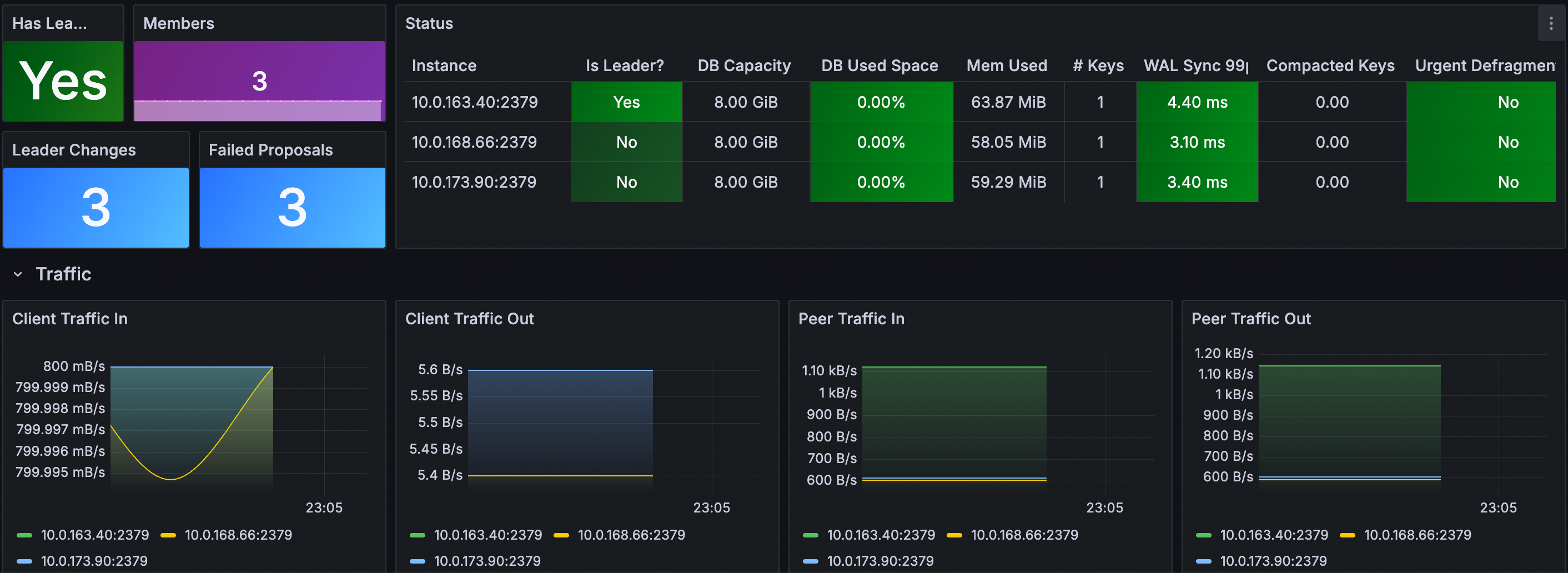
## ⚠️ Defrag - Critical Warning
Defragmentation is a HIGH-RISK operation that can severely impact your ETCD cluster and dependent systems (like GreptimeDB):
1. Blocks ALL read/write operations during execution (cluster becomes unavailable).
2. High I/O usage may cause timeouts in client applications.
3. May trigger leader elections if defrag takes too long.
4. Can cause OOM kills if not properly resourced.
5. May corrupt data if interrupted mid-process.
ETCD uses a multi-version concurrency control (MVCC) mechanism that stores multiple versions of KV. Over time, as data is updated and deleted, the backend database can become fragmented, leading to increased storage usage and reduced performance. Defragmentation is the process of compacting this storage to reclaim space and improve performance.
Add the following defrag-related configuration to `etcd-defrag.yaml` file:
```yaml
global:
security:
allowInsecureImages: true
replicaCount: 3
image:
registry: docker.io
repository: greptime/etcd
tag: 3.6.1-debian-12-r3
auth:
rbac:
create: false
token:
enabled: false
persistence:
storageClass: null
size: 8Gi
resources:
limits:
cpu: '2'
memory: 8Gi
requests:
cpu: '2'
memory: 8Gi
autoCompactionMode: "periodic"
autoCompactionRetention: "1h"
extraEnvVars:
- name: ETCD_QUOTA_BACKEND_BYTES
value: "8589934592"
- name: ETCD_ELECTION_TIMEOUT
value: "2000"
- name: ETCD_SNAPSHOT_COUNT
value: "10000"
# Defragmentation settings
defrag:
enabled: true
cronjob:
schedule: "0 3 * * *" # Daily at 3:00 AM
suspend: false
successfulJobsHistoryLimit: 1
failedJobsHistoryLimit: 1
```
Deploying with Defrag Configuration:
```bash
helm upgrade --install etcd \
oci://registry-1.docker.io/bitnamicharts/etcd \
--create-namespace \
--version 12.0.8 \
-n etcd-cluster \
--values etcd-defrag.yaml
```
You can see the etcd defrag scheduled task:
```bash
kubectl get cronjob -n etcd-cluster
```
Expected Output
```bash
NAME SCHEDULE TIMEZONE SUSPEND ACTIVE LAST SCHEDULE AGE
etcd-defrag 0 3 * * * False 0 34s
```
```bash
kubectl get pod -n etcd-cluster
```
Expected Output
```bash
NAME READY STATUS RESTARTS AGE
etcd-0 1/1 Running 0 4m30s
etcd-1 1/1 Running 0 4m29s
etcd-2 1/1 Running 0 4m29s
etcd-defrag-29128518-sstbf 0/1 Completed 0 90s
```
```bash
kubectl logs etcd-defrag-29128518-sstbf -n etcd-cluster
```
Expected Output
```log
Finished defragmenting etcd member[http://etcd-0.etcd-headless.etcd-cluster.svc.cluster.local:2379]
Finished defragmenting etcd member[http://etcd-1.etcd-headless.etcd-cluster.svc.cluster.local:2379]
Finished defragmenting etcd member[http://etcd-2.etcd-headless.etcd-cluster.svc.cluster.local:2379]
```
---
## GreptimeDB Metasrv Metadata Management Overview
# Overview
GreptimeDB cluster Metasrv component requires a metadata storage to store metadata. GreptimeDB offers flexible metadata storage options with [etcd](https://etcd.io/), [MySQL](https://www.mysql.com/), and [PostgreSQL](https://www.postgresql.org/). Each option is designed for different deployment scenarios, balancing factors like scalability, reliability, and operational overhead.
- [etcd](https://etcd.io/): A lightweight distributed key-value store perfect for metadata management. Its simplicity and ease of setup make it an excellent choice for development and testing environments.
- [MySQL](https://www.mysql.com/) and [PostgreSQL](https://www.postgresql.org/): Enterprise-grade relational databases that deliver robust metadata storage capabilities. They provide essential features including ACID transactions, replication, and comprehensive backup solutions, making them ideal for production environments. Both are widely available as managed database services (RDS) across major cloud platforms.
## Recommendation
For test and development environments, [etcd](https://etcd.io/) provides a lightweight and straightforward metadata storage solution.
**For production deployments, we strongly recommend using cloud providers' Relational Database Service (RDS) for metadata storage.** This approach offers several advantages:
- Managed service with built-in high availability and disaster recovery
- Automated backups and maintenance
- Professional monitoring and support
- Reduced operational complexity compared to self-hosted solutions
- Seamless integration with other cloud services
## Best Practices
- Implement regular backup schedules for your metadata storage
- Set up comprehensive monitoring for storage health and performance metrics
- Establish clear disaster recovery procedures
- Document your metadata storage configuration and maintenance procedures
## Next steps
- To configure the metadata storage backend, please refer to [Configuration](/user-guide/deployments-administration/manage-metadata/configuration.md).
- To setup etcd for testing and development environments, please refer to [Manage etcd](/user-guide/deployments-administration/manage-metadata/manage-etcd.md).
---
## Backup and Restore, Migrate
GreptimeDB provides metadata backup and restore capabilities through its CLI tool. This functionality supports all major metadata storage backends including etcd, MySQL, and PostgreSQL. For detailed instructions on using these features, refer to the [Backup and Restore](/user-guide/deployments-administration/disaster-recovery/back-up-&-restore-data.md) guide.
## Backup
For optimal backup reliability, schedule metadata backups during periods of low DDL (Data Definition Language) activity. This helps ensure data consistency and reduces the risk of partial or incomplete backups.
To perform a backup:
1. Verify that your GreptimeDB cluster is operational
2. Execute the backup using the CLI tool, follows the export metadata steps in [Backup and Restore](/user-guide/deployments-administration/disaster-recovery/back-up-&-restore-meta-data.md) guide.
3. Ensure the backup output file is created, and the file size is greater than 0.
## Restore
To restore from a backup:
1. Use the CLI tool to restore the metadata, follows the import metadata steps in [Backup and Restore](/user-guide/deployments-administration/disaster-recovery/back-up-&-restore-meta-data.md) guide.
2. Restart the GreptimeDB cluster to apply the restored metadata.
3. Set the [Next Table ID](/user-guide/deployments-administration/maintenance/sequence-management.md) to the original cluster's next table ID.
4. Call the [Table Reconciliation](/user-guide/deployments-administration/maintenance/table-reconciliation.md) function to repair the table metadata inconsistency.
## Migrate
We recommend to migrate metadata during periods of low DDL (Data Definition Language) activity to ensure data consistency and minimize the risk of partial or incomplete migrations.
Migrate metadata from one metadata storage to another.
1. Backup the metadata from the source storage.
2. Restore the metadata to the target storage.
3. Restart the whole GreptimeDB cluster(all components) to apply the restored metadata.
---
## Check GreptimeDB Status
GreptimeDB provides a series of HTTP endpoints to query the operational status of GreptimeDB.
The following HTTP requests assume that GreptimeDB is running on node `127.0.0.1` with the HTTP service listening on the default port `4000`.
## Check if GreptimeDB is running normally
You can use the `/health` endpoint to check if GreptimeDB is running normally.
An HTTP status code `200 OK` indicates that GreptimeDB is running normally.
Example:
```bash
curl -i -X GET http://127.0.0.1:4000/health
```
Output:
```text
HTTP/1.1 200 OK
content-type: application/json
vary: origin, access-control-request-method, access-control-request-headers
access-control-allow-origin: *
content-length: 2
date: Sun, 26 Apr 2026 13:46:41 GMT
{}
```
For more information about the health check endpoint, please refer to [the Health endpoint](/reference/http-endpoints.md#health-check).
## Check GreptimeDB status
You can use the `/status` endpoint to check the deployment status of GreptimeDB.
```bash
curl -X GET http://127.0.0.1:4000/status | jq
```
Output:
```json
{
"commit": "8d2f92c01ae762287a3cac587156519a536ae134",
"branch": "",
"rustc_version": "rustc 1.96.0-nightly (ac7f9ec7d 2026-03-20)",
"hostname": "127.0.0.1",
"version": "1.0.1"
}
```
Please refer to [the Status endpoint](/reference/http-endpoints.md#status) for more details.
---
## Self-Monitoring GreptimeDB Clusters
Before reading this document, ensure you understand how to [deploy a GreptimeDB cluster on Kubernetes](/user-guide/deployments-administration/deploy-on-kubernetes/deploy-greptimedb-cluster.md).
This guide will walk you through configuring monitoring when deploying a GreptimeDB cluster.
## Quick Start
You can enable monitoring and Grafana by adding configurations to the `values.yaml` file when deploying the GreptimeDB cluster using Helm Chart.
Here's a complete example of `values.yaml` for deploying a minimal GreptimeDB cluster with monitoring and Grafana:
```yaml
image:
# Image registry:
# Use `docker.io` for OSS GreptimeDB,
# consult staff for Enterprise GreptimeDB
registry:
# Image repository:
# Use `greptime/greptimedb` for OSS GreptimeDB
# Consult staff for GreptimeDB Enterprise
repository:
# Image tag:
# Use database version `v1.0.2` for OSS GreptimeDB
# Consult staff for GreptimeDB Enterprise
tag:
pullSecrets: []
initializer:
registry: docker.io
repository: greptime/greptimedb-initializer
tag: "v0.5.6"
monitoring:
# Enable monitoring
enabled: true
grafana:
# Enable Grafana deployment
# Requires monitoring to be enabled first (monitoring.enabled: true)
enabled: true
frontend:
replicas: 1
meta:
replicas: 1
backendStorage:
etcd:
endpoints: ["etcd.etcd-cluster.svc.cluster.local:2379"]
datanode:
replicas: 1
flownode:
replicas: 1
```
When `monitoring` is enabled, GreptimeDB Operator launches an additional GreptimeDB Standalone instance to collect metrics and logs from the GreptimeDB cluster.
To collect log data, GreptimeDB Operator starts a [Vector](https://vector.dev/) sidecar container in each Pod.
When `grafana` is enabled, a Grafana instance is deployed that uses the GreptimeDB Standalone instance configured for cluster monitoring as its data source.
This enables visualization of the GreptimeDB cluster's monitoring data out of the box using both Prometheus and MySQL protocols.
Then install the GreptimeDB cluster with the above `values.yaml` file:
```bash
helm upgrade --install mycluster \
greptime/greptimedb-cluster \
--values /path/to/values.yaml \
-n default
```
After installation, you can check the Pod status of the GreptimeDB cluster:
```bash
kubectl -n default get pods
```
Expected Output
```bash
NAME READY STATUS RESTARTS AGE
mycluster-datanode-0 2/2 Running 0 77s
mycluster-flownode-0 2/2 Running 0 2m26s
mycluster-frontend-6ffdd549b-9s7gx 2/2 Running 0 66s
mycluster-grafana-675b64786-ktqps 1/1 Running 0 6m35s
mycluster-meta-58bc88b597-ppzvj 2/2 Running 0 86s
mycluster-monitor-standalone-0 1/1 Running 0 6m35s
```
You can then access the Grafana dashboard by port-forwarding the Grafana service to your local machine:
```shell
kubectl -n default port-forward svc/mycluster-grafana 18080:80
```
Then refer to the [Access Grafana Dashboard](#access-grafana-dashboard) section below for details on accessing Grafana.
## Monitoring Configuration
This section covers the details of monitoring configurations.
### Enable Monitoring
Add the following configuration to [`values.yaml`](/user-guide/deployments-administration/deploy-on-kubernetes/deploy-greptimedb-cluster.md#setup-valuesyaml) to enable monitoring when deploying the GreptimeDB cluster:
```yaml
monitoring:
enabled: true
```
This deploys a GreptimeDB Standalone instance named `${cluster-name}-monitoring` to collect metrics and logs. You can verify the deployment with:
```bash
kubectl get greptimedbstandalones.greptime.io ${cluster-name}-monitoring -n ${namespace}
```
The GreptimeDB Standalone instance exposes services using `${cluster-name}-monitoring-standalone` as the Kubernetes Service name. You can use the following addresses to access monitoring data:
- **Prometheus metrics**: `http://${cluster-name}-monitor-standalone.${namespace}.svc.cluster.local:4000/v1/prometheus`
- **SQL logs**: `${cluster-name}-monitor-standalone.${namespace}.svc.cluster.local:4002`. By default, cluster logs are stored in the `public._gt_logs` table.
### Customize Monitoring Storage
By default, the GreptimeDB Standalone instance stores monitoring data using the Kubernetes default StorageClass in local storage.
You can configure the GreptimeDB Standalone instance through the `monitoring.standalone` field in `values.yaml`. For example, the following configuration uses S3 object storage to store monitoring data:
```yaml
monitoring:
enabled: true
standalone:
base:
main:
# Configure GreptimeDB Standalone instance image
image: "greptime/greptimedb:v1.0.2"
# Configure GreptimeDB Standalone instance resources
resources:
requests:
cpu: "2"
memory: "4Gi"
limits:
cpu: "2"
memory: "4Gi"
# Configure object storage for GreptimeDB Standalone instance
objectStorage:
s3:
# Configure bucket
bucket: "monitoring"
# Configure region
region: "ap-southeast-1"
# Configure secret name
secretName: "s3-credentials"
# Configure root path
root: "standalone-with-s3-data"
```
### Customize Vector Sidecar
The Vector sidecar configuration for log collection can be customized via the `monitoring.vector` field.
For example, you can adjust the Vector image and resource limits as follows:
```yaml
monitoring:
enabled: true
vector:
# Configure Vector image registry
registry: docker.io
# Configure Vector image repository
repository: timberio/vector
# Configure Vector image tag
tag: nightly-alpine
# Configure Vector resources
resources:
requests:
cpu: "50m"
memory: "64Mi"
limits:
cpu: "50m"
memory: "64Mi"
```
### YAML Configuration with `kubectl` Deployment
If you're not using Helm Chart, you can also use the `monitoring` field to manually configure self-monitoring mode in the `GreptimeDBCluster` YAML:
```yaml
monitoring:
enabled: true
```
For detailed configuration options, refer to the [`GreptimeDBCluster` API documentation](https://github.com/GreptimeTeam/greptimedb-operator/blob/main/docs/api-references/docs.md#monitoringspec).
## Grafana Configuration
### Enable Grafana
To enable Grafana deployment, add the following configuration to `values.yaml`.
Note that monitoring must be enabled first [(`monitoring.enabled: true`)](#enable-monitoring):
```yaml
monitoring:
enabled: true
grafana:
enabled: true
```
### Customize Grafana Data Sources
By default, Grafana uses `mycluster` and `default` as the cluster name and namespace to create data sources.
To monitor clusters with different names or namespaces, you need to create custom data source configurations based on the actual cluster names and namespaces.
Here's an example `values.yaml` configuration:
```yaml
monitoring:
enabled: true
grafana:
enabled: true
datasources:
datasources.yaml:
datasources:
# Query the cluster metrics.
- name: greptimedb-metrics
type: prometheus
url: http://${cluster-name}-monitor-standalone.${namespace}.svc.cluster.local:4000/v1/prometheus
access: proxy
# Query the cluster traces.
- name: greptimedb-traces
type: jaeger
url: http://${cluster-name}-monitor-standalone.${namespace}.svc.cluster.local:4000/v1/jaeger
access: proxy
# Query the cluster logs and slow queries.
- name: greptimedb-logs
type: mysql
url: ${cluster-name}-monitor-standalone.${namespace}.svc.cluster.local:4002
access: proxy
database: public
# Query the information schema from the cluster.
- name: information_schema
type: mysql
url: ${cluster-name}-frontend.${namespace}.svc.cluster.local:4002
access: proxy
database: information_schema
```
This configuration creates the following data sources for GreptimeDB cluster monitoring in Grafana:
- **`greptimedb-metrics`**: Cluster metrics stored in the standalone monitoring database, exposed via Prometheus protocol (`type: prometheus`)
- **`greptimedb-logs`**: Cluster logs stored in the standalone monitoring database, exposed via MySQL protocol (`type: mysql`). Uses the `public` database by default
- **`greptimedb-traces`**: Cluster traces stored in the standalone monitoring database, exposed via Jaeger protocol (`type: jaeger`). Uses the `public` database by default
- **`information_schema`**: Cluster information stored in the frontend database, exposed via MySQL protocol (`type: mysql`). Uses the `information_schema` database by default
### Access Grafana Dashboard
You can access the Grafana dashboard by port-forwarding the Grafana service to your local machine:
```bash
kubectl -n ${namespace} port-forward svc/${cluster-name}-grafana 18080:80
```
Then open `http://localhost:18080` to access the Grafana dashboard.
The default login credentials for Grafana are:
- **Username**: `admin`
- **Password**: `gt-operator`
Navigate to the `Dashboards` section to explore the pre-configured dashboards for monitoring your GreptimeDB cluster.
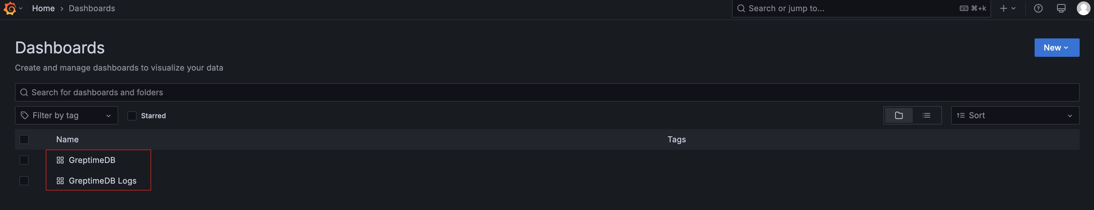
## Cleanup the PVCs
:::danger
The cleanup operation will remove the metadata and data of the GreptimeDB cluster. Please make sure you have backed up the data before proceeding.
:::
To uninstall the GreptimeDB cluster, please refer to the [Cleanup GreptimeDB Cluster](/user-guide/deployments-administration/deploy-on-kubernetes/deploy-greptimedb-cluster.md#cleanup) documentation.
To clean up the Persistent Volume Claims (PVCs) used by the GreptimeDB standalone monitoring instance, delete the PVCs using the following command:
```bash
kubectl -n default delete pvc -l app.greptime.io/component=${cluster-name}-monitor-standalone
```
---
## Key Logs
During operation, GreptimeDB outputs key operations and unexpected error information to logs.
You can use these logs to understand GreptimeDB's operational status and troubleshoot errors.
## Log Location
GreptimeDB components default to outputting INFO level logs to the following locations:
- Standard output
- `greptimedb_data/logs` directory under GreptimeDB's current working directory
The log output directory can also be modified through the `[logging]` section in the configuration file or the `--log_dir` startup parameter:
```toml
[logging]
dir = "/path/to/logs"
```
Log file formats are:
- `greptimedb.YYYY-MM-DD-HH` contains logs of INFO level and above
- `greptimedb-err.YYYY-MM-DD-HH` contains error logs
For example:
```bash
greptimedb.2025-04-11-06
greptimedb-err.2025-04-11-06
```
Currently, GreptimeDB components include:
- frontend
- datanode
- metasrv
- flownode
If you need to adjust log levels, such as viewing DEBUG level logs for a component, you can refer to [this document](https://github.com/GreptimeTeam/greptimedb/blob/main/docs/how-to/how-to-change-log-level-on-the-fly.md) to modify them at runtime.
## Important Logs
The following lists recommended logs to monitor:
### Error Logs
When the database is running normally and stably, it will not output error logs. If database operations encounter exceptions or panics occur, error logs will be printed. It is recommended that users check error logs from all components.
#### Panic
If the database encounters a panic, it is recommended to collect the panic logs and report them to the official team. Typical panic logs look like this, with the keyword `panicked at`:
```bash
2025-04-02T14:44:24.485935Z ERROR common_telemetry::panic_hook: panicked at /greptime/.cargo/git/checkouts/datafusion-11a8b534adb6bd68-shallow/2464703/datafusion/expr/src/logical_plan/plan.rs:1035:25:
with_new_exprs for Distinct does not support sort expressions backtrace= 0: backtrace::backtrace::libunwind::trace
at /greptime/.cargo/registry/src/index.crates.io-1949cf8c6b5b557f/backtrace-0.3.74/src/backtrace/libunwind.rs:116:5
backtrace::backtrace::trace_unsynchronized
at /greptime/.cargo/registry/src/index.crates.io-1949cf8c6b5b557f/backtrace-0.3.74/src/backtrace/mod.rs:66:5
1: backtrace::backtrace::trace
at /greptime/.cargo/registry/src/index.crates.io-1949cf8c6b5b557f/backtrace-0.3.74/src/backtrace/mod.rs:53:14
2: backtrace::capture::Backtrace::create
at /greptime/.cargo/registry/src/index.crates.io-1949cf8c6b5b557f/backtrace-0.3.74/src/capture.rs:292:9
3: backtrace::capture::Backtrace::new
at /greptime/.cargo/registry/src/index.crates.io-1949cf8c6b5b557f/backtrace-0.3.74/src/capture.rs:257:22
4: common_telemetry::panic_hook::set_panic_hook::{{closure}}
at /greptime/codes/greptime/procedure-traits/src/common/telemetry/src/panic_hook.rs:37:25
5: as core::ops::function::Fn>::call
at /rustc/409998c4e8cae45344fd434b358b697cc93870d0/library/alloc/src/boxed.rs:1984:9
std::panicking::rust_panic_with_hook
at /rustc/409998c4e8cae45344fd434b358b697cc93870d0/library/std/src/panicking.rs:820:13
6: std::panicking::begin_panic_handler::{{closure}}
at /rustc/409998c4e8cae45344fd434b358b697cc93870d0/library/std/src/panicking.rs:678:13
7: std::sys::backtrace::__rust_end_short_backtrace
at /rustc/409998c4e8cae45344fd434b358b697cc93870d0/library/std/src/sys/backtrace.rs:168:18
8: rust_begin_unwind
at /rustc/409998c4e8cae45344fd434b358b697cc93870d0/library/std/src/panicking.rs:676:5
9: core::panicking::panic_fmt
at /rustc/409998c4e8cae45344fd434b358b697cc93870d0/library/core/src/panicking.rs:75:14
10: datafusion_expr::logical_plan::plan::LogicalPlan::with_new_exprs
at /greptime/.cargo/git/checkouts/datafusion-11a8b534adb6bd68-shallow/2464703/datafusion/expr/src/logical_plan/plan.rs:1035:25
11: ::analyze::{{closure}}
at /greptime/codes/greptime/procedure-traits/src/query/src/optimizer/type_conversion.rs:105:17
12: core::ops::function::impls::::call_mut
at /greptime/.rustup/toolchains/nightly-2024-12-25-aarch64-apple-darwin/lib/rustlib/src/rust/library/core/src/ops/function.rs:272:13
13: core::ops::function::impls::::call_once
at /greptime/.rustup/toolchains/nightly-2024-12-25-aarch64-apple-darwin/lib/rustlib/src/rust/library/core/src/ops/function.rs:305:13
14: datafusion_common::tree_node::Transformed::transform_parent
at /greptime/.cargo/git/checkouts/datafusion-11a8b534adb6bd68-shallow/2464703/datafusion/common/src/tree_node.rs:764:44
15: datafusion_common::tree_node::TreeNode::transform_up::transform_up_impl::{{closure}}
at /greptime/.cargo/git/checkouts/datafusion-11a8b534adb6bd68-shallow/2464703/datafusion/common/src/tree_node.rs:265:13
16: stacker::maybe_grow
at /greptime/.cargo/registry/src/index.crates.io-1949cf8c6b5b557f/stacker-0.1.17/src/lib.rs:55:9
datafusion_common::tree_node::TreeNode::transform_up::transform_up_impl
at /greptime/.cargo/git/checkouts/datafusion-11a8b534adb6bd68-shallow/2464703/datafusion/common/src/tree_node.rs:260:9
17: datafusion_common::tree_node::TreeNode::transform_up
at /greptime/.cargo/git/checkouts/datafusion-11a8b534adb6bd68-shallow/2464703/datafusion/common/src/tree_node.rs:269:9
18: datafusion_common::tree_node::TreeNode::transform
at /greptime/.cargo/git/checkouts/datafusion-11a8b534adb6bd68-shallow/2464703/datafusion/common/src/tree_node.rs:220:9
19: ::analyze
at /greptime/codes/greptime/procedure-traits/src/query/src/optimizer/type_conversion.rs:46:9
20: query::query_engine::state::QueryEngineState::optimize_by_extension_rules::{{closure}}
at /greptime/codes/greptime/procedure-traits/src/query/src/query_engine/state.rs:195:17
21: core::iter::traits::iterator::Iterator::try_fold
at /greptime/.rustup/toolchains/nightly-2024-12-25-aarch64-apple-darwin/lib/rustlib/src/rust/library/core/src/iter/traits/iterator.rs:2370:21
22: query::query_engine::state::QueryEngineState::optimize_by_extension_rules
at /greptime/codes/greptime/procedure-traits/src/query/src/query_engine/state.rs:192:9
23: query::planner::DfLogicalPlanner::plan_sql::{{closure}}::{{closure}}
at /greptime/codes/greptime/procedure-traits/src/query/src/planner.rs:119:20
24: as core::future::future::Future>::poll
at /greptime/.cargo/registry/src/index.crates.io-1949cf8c6b5b557f/tracing-0.1.40/src/instrument.rs:321:9
25: query::planner::DfLogicalPlanner::plan_sql::{{closure}}
at /greptime/codes/greptime/procedure-traits/src/query/src/planner.rs:71:5
26: ::plan::{{closure}}::{{closure}}
at /greptime/codes/greptime/procedure-traits/src/query/src/planner.rs:198:73
27: as core::future::future::Future>::poll
at /greptime/.cargo/registry/src/index.crates.io-1949cf8c6b5b557f/tracing-0.1.40/src/instrument.rs:321:9
28: ::plan::{{closure}}
at /greptime/codes/greptime/procedure-traits/src/query/src/planner.rs:195:5
...
```
### Metasrv
When the GreptimeDB cluster experiences node online/offline events,
region migration, schema changes, etc.,
metasrv will record corresponding logs.
Therefore, in addition to error logs from each component,
it is also recommended to monitor the following metasrv log keywords:
#### Metasrv Leader Step Down/Election
```bash
// Error level, indicates current leader stepped down, new election will follow. Note the {:?} part is the leader identifier
"Leader :{:?} step down"
```
#### Region Lease Renewal Failure
```bash
// Warning level, indicates a region lease renewal was denied. Region lease requests will be rejected when the region is not properly closed/scheduled on a datanode.
Denied to renew region lease for datanode: {datanode_id}, region_id: {region_id}
```
```bash
// Info level, datanode receives lease renewal failure and attempts to close target region
Closing staled region:
```
#### Region Failover
```bash
// Warning level, detects some regions failed Phi health check, need to execute failover operation. Region IDs will be printed after the colon
Detects region failures:
// A region migration failed
Failed to wait region migration procedure
// Info level, when maintenance mode is enabled, failover procedure will be skipped
Maintenance mode is enabled, skip failover
```
#### Region Migration
```bash
// Info level, indicates a region starts migration. Region information will be printed after the log
Starting region migration procedure
// Error level, a region migration failed
Failed to wait region migration procedure
```
#### Procedure
Metasrv internally uses a component called "procedure" to execute distributed operations. You can monitor error logs from this component:
```bash
Failed to execute procedure
```
#### Flow Creation Failure
When flow creation fails, the failure reason can usually be seen in procedure error logs. Logs may contain the following keywords:
```bash
Failed to execute procedure metasrv-procedure:: CreateFlow
```
### Datanode
#### Compaction
When compaction starts and ends, datanode will log the following information:
```bash
2025-05-16T06:01:08.794415Z INFO mito2::compaction::task: Compacted SST files, region_id: 4612794875904(1074, 0), input: [FileMeta { region_id: 4612794875904(1074, 0), file_id: FileId(a29500fb-cae0-4f3f-8376-cb3f14653378), time_range: (1686455010000000000::Nanosecond, 1686468410000000000::Nanosecond), level: 0, file_size: 45893329, available_indexes: [], index_file_size: 0, num_rows: 5364000, num_row_groups: 53, sequence: Some(114408000) }, FileMeta { region_id: 4612794875904(1074, 0), file_id: FileId(a31dcb1b-19ae-432f-8482-9e1b7db7b53b), time_range: (1686468420000000000::Nanosecond, 1686481820000000000::Nanosecond), level: 0, file_size: 45900506, available_indexes: [], index_file_size: 0, num_rows: 5364000, num_row_groups: 53, sequence: Some(119772000) }], output: [FileMeta { region_id: 4612794875904(1074, 0), file_id: FileId(5d105ca7-9e3c-4298-afb3-e85baae3b2e8), time_range: (1686455010000000000::Nanosecond, 1686481820000000000::Nanosecond), level: 1, file_size: 91549797, available_indexes: [], index_file_size: 0, num_rows: 10728000, num_row_groups: 105, sequence: Some(119772000) }], window: Some(86400), waiter_num: 0, merge_time: 3.034328293s
```
```bash
2025-05-16T06:01:08.805366Z INFO mito2::request: Successfully compacted region: 4612794875904(1074, 0)
```
---
## Prometheus-Monitoring GreptimeDB Cluster
Before reading this document, ensure you understand how to [deploy a GreptimeDB cluster on Kubernetes](/user-guide/deployments-administration/deploy-on-kubernetes/deploy-greptimedb-cluster.md).
It is recommended to use [self-monitoring mode](cluster-monitoring-deployment.md) to monitor GreptimeDB cluster,
as it's simple to set up and provides out-of-the-box Grafana dashboards.
However, if you already have a Prometheus instance deployed in your Kubernetes cluster and want to integrate
GreptimeDB cluster metrics into it, follow the steps below.
## Check the Prometheus Instance Configuration
Ensure you have deployed the Prometheus Operator and created a Prometheus instance. For example, you can use [kube-prometheus-stack](https://github.com/prometheus-community/helm-charts/tree/main/charts/kube-prometheus-stack) to deploy the Prometheus stack. Refer to its [official documentation](https://github.com/prometheus-community/helm-charts/tree/main/charts/kube-prometheus-stack) for more details.
When deploying the Prometheus instance, ensure you set the labels used for scraping GreptimeDB cluster metrics.
For example, your existing Prometheus instance may contain the following configuration:
```yaml
apiVersion: monitoring.coreos.com/v1
kind: PodMonitor
metadata:
name: greptime-podmonitor
namespace: default
spec:
selector:
matchLabels:
release: prometheus
# other configurations...
```
When the `PodMonitor` is deployed,
the Prometheus Operator continuously watches for pods in the `default` namespace that match all labels defined in `spec.selector.matchLabels` (in this example, `release: prometheus`).
## Enable `prometheusMonitor` for GreptimeDB Cluster
When deploying a GreptimeDB cluster using a Helm Chart,
enable the `prometheusMonitor` field in your `values.yaml` file. For example:
```yaml
prometheusMonitor:
# Enable Prometheus monitoring - this will create PodMonitor resources
enabled: true
# Configure scrape interval
interval: "30s"
# Configure labels
labels:
release: prometheus
```
**Important:** The `labels` field value (`release: prometheus`)
must match the `matchLabels` field used to create the Prometheus instance,
otherwise metrics collection won't work properly.
After configuring `prometheusMonitor`,
the GreptimeDB Operator will automatically create `PodMonitor` resources and import metrics into Prometheus at the specified `interval`.
You can check the `PodMonitor` resources with:
```
kubectl get podmonitors.monitoring.coreos.com -n ${namespace}
```
:::note
If you're not using a Helm Chart, you can manually configure Prometheus monitoring in the `GreptimeDBCluster` YAML:
```yaml
apiVersion: greptime.io/v1alpha1
kind: GreptimeDBCluster
metadata:
name: basic
spec:
base:
main:
image: greptime/greptimedb:v1.0.2
frontend:
replicas: 1
meta:
replicas: 1
backendStorage:
etcd:
endpoints:
- "etcd.etcd-cluster.svc.cluster.local:2379"
datanode:
replicas: 1
prometheusMonitor:
enabled: true
interval: "30s"
labels:
release: prometheus
```
:::
## Grafana Dashboards
You need to deploy Grafana by yourself,
then import the dashboards.
### Add Data Sources
After deploying Grafana,
refer to Grafana's [data sources](https://grafana.com/docs/grafana/latest/datasources/) documentation to add the following two type data sources:
- **Prometheus**: Name it `metrics`. This data source connects to your Prometheus instance, which collects GreptimeDB cluster monitoring metrics. Use your Prometheus instance URL as the connection URL.
- **MySQL**: Name it `information-schema`. This data source connects to your GreptimeDB cluster to access cluster metadata via the SQL protocol. If you have deployed GreptimeDB following the [Deploy a GreptimeDB Cluster on Kubernetes](/user-guide/deployments-administration/deploy-on-kubernetes/deploy-greptimedb-cluster.md) guide, use `${cluster-name}-frontend.${namespace}.svc.cluster.local:4002` as the server address with database `information_schema`.
### Import Dashboards
The [GreptimeDB Cluster Metrics Dashboard](https://github.com/GreptimeTeam/greptimedb/tree/v1.0.2/grafana/dashboards/metrics/cluster) uses the `metrics` and `information-schema` data sources to display GreptimeDB cluster metrics.
Refer to Grafana's [Import dashboards](https://grafana.com/docs/grafana/latest/dashboards/build-dashboards/import-dashboards/) documentation to learn how to import dashboards.
---
## Monitoring
Effective database administration relies heavily on monitoring.
You can monitor GreptimeDB using the following methods:
---
## Runtime Information
The `INFORMATION_SCHEMA` database provides access to system metadata, such as the name of a database or table, the data type of a column, etc.
* Find the topology information of the cluster though [CLUSTER_INFO](/reference/sql/information-schema/cluster-info.md) table.
* Find the table regions distribution though [PARTITIONS](/reference/sql/information-schema/partitions.md) and [REGION_PEERS](/reference/sql/information-schema/region-peers.md) tables.
For example, find all the region id of a table:
```sql
SELECT greptime_partition_id FROM PARTITIONS WHERE table_name = 'monitor'
```
Find the distribution of all regions in a table:
```sql
SELECT b.peer_id as datanode_id,
a.greptime_partition_id as region_id
FROM information_schema.partitions a LEFT JOIN information_schema.region_peers b
ON a.greptime_partition_id = b.region_id
WHERE a.table_name='monitor'
ORDER BY datanode_id ASC
```
For more information about the `INFORMATION_SCHEMA` database,
Please read the [reference](/reference/sql/information-schema/overview.md).
---
## Slow Query (Experimental)
GreptimeDB provides a slow query log to help you find and fix slow queries. By default, the slow queries are output to the system table `greptime_private.slow_queries` with `30s` threshold and `1.0` sample ratio with `30d` TTL.
The schema of the `greptime_private.slow_queries` table is as follows:
```sql
+--------------+----------------------+------+------+---------+---------------+
| Column | Type | Key | Null | Default | Semantic Type |
+--------------+----------------------+------+------+---------+---------------+
| cost | UInt64 | | NO | | FIELD |
| threshold | UInt64 | | NO | | FIELD |
| query | String | | NO | | FIELD |
| is_promql | Boolean | | NO | | FIELD |
| timestamp | TimestampNanosecond | PRI | NO | | TIMESTAMP |
| promql_range | UInt64 | | NO | | FIELD |
| promql_step | UInt64 | | NO | | FIELD |
| promql_start | TimestampMillisecond | | NO | | FIELD |
| promql_end | TimestampMillisecond | | NO | | FIELD |
+--------------+----------------------+------+------+---------+---------------+
```
- `cost`: The cost of the query in milliseconds.
- `threshold`: The threshold of the query in milliseconds.
- `query`: The query string.
- `is_promql`: Whether the query is a PromQL query.
- `timestamp`: The timestamp of the query.
- `promql_range`: The range of the query. Only used when `is_promql` is `true`.
- `promql_step`: The step of the query. Only used when `is_promql` is `true`.
- `promql_start`: The start time of the query. Only used when `is_promql` is `true`.
- `promql_end`: The end time of the query. Only used when `is_promql` is `true`.
In cluster mode, you can configure the slow query in frontend configs (same as in standalone mode), for example:
```toml
[slow_query]
## Whether to enable slow query log.
enable = true
## The record type of slow queries. It can be `system_table` or `log`.
## If `system_table` is selected, the slow queries will be recorded in a system table `greptime_private.slow_queries`.
## If `log` is selected, the slow queries will be logged in a log file `greptimedb-slow-queries.*`.
record_type = "system_table"
## The threshold of slow query. It can be human readable time string, for example: `10s`, `100ms`, `1s`.
threshold = "30s"
## The sampling ratio of slow query log. The value should be in the range of (0, 1]. For example, `0.1` means 10% of the slow queries will be logged and `1.0` means all slow queries will be logged.
sample_ratio = 1.0
## The TTL of the `slow_queries` system table. Default is `30d` when `record_type` is `system_table`.
ttl = "30d"
```
If you use the Helm chart to deploy GreptimeDB, you can configure the slow query in the `values.yaml` file, for example:
```yaml
slowQuery:
enable: true
recordType: "system_table"
threshold: "30s"
sampleRatio: "1.0"
ttl: "30d"
```
If you use `log` as the record type, the slow queries will be logged in a log file `greptimedb-slow-queries.*`. By default, the log file is located in the `${data_home}/logs` directory.
---
## Standalone Monitoring
GreptimeDB standalone provides a `/metrics` endpoint on the HTTP port (default `4000`) that exposes [Prometheus metrics](/reference/http-endpoints.md#metrics).
You can use Prometheus to scrape these metrics and Grafana to visualize them.
## Grafana Dashboard Integration
GreptimeDB provides pre-built Grafana dashboards for monitoring standalone deployments.
You can access the dashboard JSON files from the [GreptimeDB repository](https://github.com/GreptimeTeam/greptimedb/tree/v1.0.2/grafana/dashboards/metrics/standalone).
---
## Tracing
GreptimeDB supports distributed tracing. GreptimeDB exports all collected spans using the gRPC-based OTLP protocol. Users can use [Jaeger](https://www.jaegertracing.io/), [Tempo](https://grafana.com/oss/tempo/) and other OTLP protocol backends that support gRPC to collect the span instrument by GreptimeDB.
In the [logging section](/user-guide/deployments-administration/configuration.md#logging-options) in the configuration, there are descriptions of configuration items related to tracing, [standalone.example.toml](https://github.com/GreptimeTeam/greptimedb/blob/v1.0.2/config/standalone.example.toml) provide a reference configuration in the logging section.
## Dynamic Tracing Control
GreptimeDB provides the ability to enable or disable tracing dynamically at runtime using the HTTP API without requiring a server restart. This is useful for troubleshooting production issues or temporarily enabling tracing for debugging purposes.
To enable tracing:
```bash
curl --data "true" http://127.0.0.1:4000/debug/enable_trace
# Output: trace enabled
```
To disable tracing:
```bash
curl --data "false" http://127.0.0.1:4000/debug/enable_trace
# Output: trace disabled
```
## Tutorial: Use Jaeger to trace GreptimeDB
[Jaeger](https://www.jaegertracing.io/) is an open source, end-to-end distributed tracing system, originally developed and open sourced by Uber. Its goal is to help developers monitor and debug the request flow in complex microservice architectures.
Jaeger supports gRPC-based OTLP protocol, so GreptimeDB can export trace data to Jaeger. The following tutorial shows you how to deploy and use Jaeger to track GreptimeDB.
### Step 1: Deploy Jaeger
Start a Jaeger instance using the `all-in-one` docker image officially provided by jaeger:
```bash
docker run --rm -d --name jaeger \
-e COLLECTOR_ZIPKIN_HOST_PORT=:9411 \
-p 6831:6831/udp \
-p 6832:6832/udp \
-p 5778:5778 \
-p 16686:16686 \
-p 4317:4317 \
-p 4318:4318 \
-p 14250:14250 \
-p 14268:14268 \
-p 14269:14269 \
-p 9411:9411 \
jaegertracing/all-in-one:latest
```
### Step 2: Deploy GreptimeDB
Write configuration files to allow GreptimeDB to perform tracing. Save the following configuration items as the file `config.toml`
```Toml
[logging]
enable_otlp_tracing = true
```
Then start GreptimeDB using standalone mode
```bash
greptime standalone start -c config.toml
```
Refer to the chapter [MySQL](/user-guide/protocols/mysql.md) on how to connect to GreptimeDB. Run the following SQL statement in MySQL Client:
```sql
CREATE TABLE host (
ts timestamp(3) time index,
host STRING PRIMARY KEY,
val BIGINT,
);
INSERT INTO TABLE host VALUES
(0, 'host1', 0),
(20000, 'host2', 5);
SELECT * FROM host ORDER BY ts;
DROP TABLE host;
```
### Step 3: Obtain trace information in Jaeger
1. Go to http://127.0.0.1:16686/ and select the Search tab.
2. Select the `greptime-standalone` service in the service drop-down list.
3. Click **Find Traces** to display trace information.
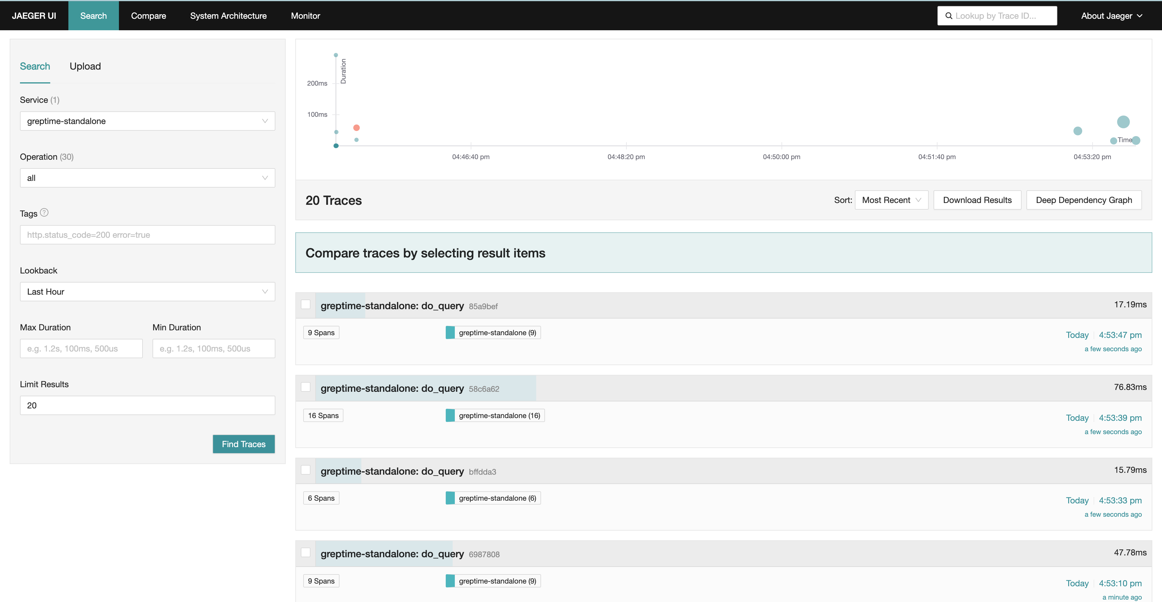
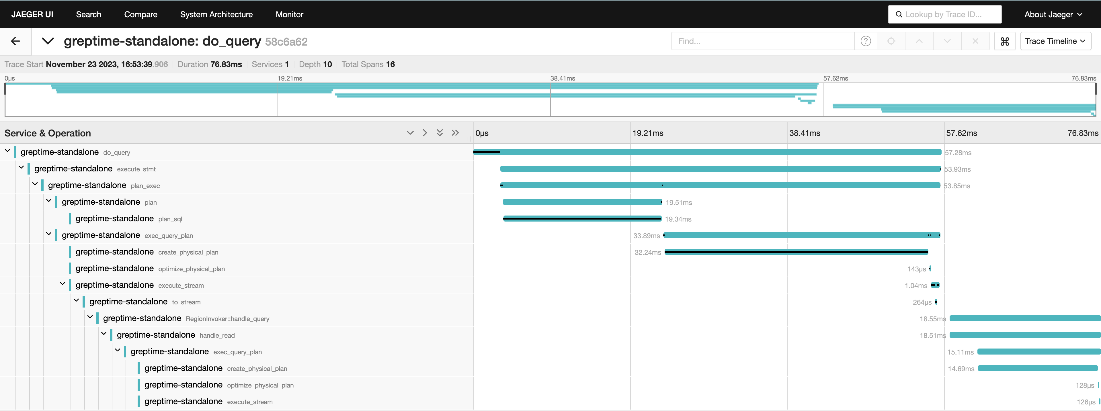
## Guide: How to configure tracing sampling rate
GreptimeDB provides many protocols and interfaces for data insertion, query and other functions. You can collect the calling chains of each operation through tracing. However, for some high-frequency operations, collecting all tracing of the operation may be unnecessary and waste storage space. At this time, you can use `tracing_sample_ratio` to set the sampling rate of tracing for various operations, which can greatly reduce the number of exported tracing and facilitate system observation.
All tracing within GreptimeDB is classified according to the protocol it is connected to and the corresponding operations of that protocol:
| **protocol** | **request_type** |
|--------------|-----------------------------------------------------------------------------------------------------------------------------------------------------------------------------------------------------------------------|
| grpc | inserts / query.sql / query.logical_plan / query.prom_range / query.empty / ddl.create_database / ddl.create_table / ddl.alter / ddl.drop_table / ddl.truncate_table / ddl.empty / deletes / row_inserts / row_deletes |
| mysql | |
| postgres | |
| otlp | metrics / traces |
| opentsdb | |
| influxdb | write_v1 / write_v2 |
| prometheus | remote_read / remote_write / format_query / instant_query / range_query / labels_query / series_query / label_values_query |
| http | sql / promql
You can configure different tracing sampling rates through `tracing_sample_ratio`.
```toml
[logging]
enable_otlp_tracing = true
[logging.tracing_sample_ratio]
default_ratio = 0.0
[[logging.tracing_sample_ratio.rules]]
protocol = "mysql"
ratio = 1.0
[[logging.tracing_sample_ratio.rules]]
protocol = "grpc"
request_types = ["inserts"]
ratio = 0.3
```
The above configuration formulates two sampling rules and sets a default sampling rate. GreptimeDB will start matching from the first one according to the sampling rules, and use the first matching sampling rule as the sampling rate of the tracing. If no rule matches, `default_ratio` will be used as the default sampling rate. The range of sampling rate is `[0.0, 1.0]`, `0.0` means not sampling, `1.0` means sampling all tracing.
For example, according to the rules provided above, all calls accessed using the mysql protocol will be sampled, data inserted using grpc will be sampled 30%, and all remaining tracing will not be sampled.
---
## Deployments & Administration
GreptimeDB can be deployed and managed either on your own infrastructure or through GreptimeCloud.
This guide provides an overview of deployment strategies, configuration, monitoring, and administration.
## GreptimeDB Architecture
Before diving into the deployment and administration of GreptimeDB,
it's important to understand its [architecture](/user-guide/concepts/architecture.md).
## Self-Managed GreptimeDB Deployment
This section outlines the key aspects of deploying and administering GreptimeDB in your own environment.
### Configuration and Deployment
- **Configuration:** Before deployment, [check the configuration](configuration.md) to suit your requirements, including protocol settings, storage options, and more.
- **Authentication:** By default, authentication is not enabled. Learn how to [enable and configure authentication](./authentication/overview.md) for secure deployments.
- **Kubernetes Deployment:** Follow the [step-by-step guide](./deploy-on-kubernetes/overview.md) to deploy GreptimeDB on Kubernetes.
- **Capacity Planning:** Ensure your deployment can handle your workload by [planning for capacity](/user-guide/deployments-administration/capacity-plan.md).
### Component Management
- **Cluster Failover:** Set up [Remote WAL](./wal/remote-wal/configuration.md) for high availability.
- **Manage Metadata:** Set up [Metadata Storage](./manage-data/overview.md) for GreptimeDB.
### Monitoring
- **Monitoring:** [Monitor cluster's health and performance](./monitoring/overview.md) through metrics, tracing, and runtime information.
### Data Management and Performance
- **Data Management:** [Manage your data](/user-guide/deployments-administration/manage-data/overview.md) to prevent data loss, reduce costs, and optimize performance.
- **Performance Tuning:** Review [performance tuning tips](/user-guide/deployments-administration/performance-tuning/performance-tuning-tips.md) and learn how to [design your table schema](/user-guide/deployments-administration/performance-tuning/design-table.md) for optimal efficiency.
### Disaster Recovery
- **Disaster Recovery:** Implement [disaster recovery strategies](/user-guide/deployments-administration/disaster-recovery/overview.md) to protect your data and ensure business continuity.
### Additional Topics
- **Run on Android:** Learn how to [run GreptimeDB on Android devices](run-on-android.md).
- **Upgrade:** Follow the [upgrade guide](/user-guide/deployments-administration/upgrade.md) to keep the version of GreptimeDB up to date.
---
## Design Your Table Schema
The design of your table schema significantly impacts both write and query performance.
Before writing data,
it is crucial to understand the data types, scale, and common queries relevant to your business,
then model the data accordingly.
This document provides a comprehensive guide on GreptimeDB's data model and table schema design for various scenarios.
## Understanding GreptimeDB's Data Model
Before proceeding, please review the GreptimeDB [Data Model Documentation](/user-guide/concepts/data-model.md).
## Basic Concepts
### Cardinality
**Cardinality**: Refers to the number of unique values in a dataset. It can be classified as "high cardinality" or "low cardinality":
- **Low Cardinality**: Low cardinality columns usually have constant values.
The total number of unique values usually no more than 10 thousand.
For example, `namespace`, `cluster`, `http_method` are usually low cardinality.
- **High Cardinality**: High cardinality columns contain a large number of unique values.
For example, `trace_id`, `span_id`, `user_id`, `uri`, `ip`, `uuid`, `request_id`, table auto increment id, timestamps are usually high cardinality.
### Column Types
In GreptimeDB, columns are categorized into three semantic types: `Tag`, `Field`, and `Timestamp`.
The timestamp usually represents the time of data sampling or the occurrence time of logs/events.
GreptimeDB uses the `TIME INDEX` constraint to identify the `Timestamp` column.
So the `Timestamp` column is also called the `TIME INDEX` column.
If you have multiple columns with timestamp data type, you can only define one as `TIME INDEX` and others as `Field` columns.
In GreptimeDB, tag columns are optional. The main purposes of tag columns include:
1. Defining the ordering of data in storage.
GreptimeDB reuses the `PRIMARY KEY` constraint to define tag columns and the ordering of tags.
Unlike traditional databases, GreptimeDB defines time-series by the primary key.
Tables in GreptimeDB sort rows in the order of `(primary key, timestamp)`.
This improves the locality of data with the same tags.
If there are no tag columns, GreptimeDB sorts rows by timestamp.
2. Identifying a unique time-series.
When the table is not append-only, GreptimeDB can deduplicate rows by timestamp under the same time-series (primary key).
3. Smoothing migration from other TSDBs that use tags or labels.
## Primary key
### Primary key is optional
Bad primary key or index may significantly degrade performance.
Generally you can create an append-only table without a primary key since ordering data by timestamp is sufficient for many workloads.
It can also serve as a baseline.
```sql
CREATE TABLE http_logs (
access_time TIMESTAMP TIME INDEX,
application STRING,
remote_addr STRING,
http_status STRING,
http_method STRING,
http_refer STRING,
user_agent STRING,
request_id STRING,
request STRING,
) with ('append_mode'='true');
```
The `http_logs` table is an example for storing HTTP server logs.
- The `'append_mode'='true'` option creates the table as an append-only table.
This ensures a log doesn't override another one with the same timestamp.
- The table sorts logs by time so it is efficient to search logs by time.
### Primary key design and SST format
You can use primary key when there are suitable columns and one of the following conditions is met:
- Most queries can benefit from the ordering.
- You need to deduplicate (including delete) rows by the primary key and time index.
For example, if you always only query logs of a specific application, you may set the `application` column as primary key (tag).
```sql
SELECT message FROM http_logs WHERE application = 'greptimedb' AND access_time > now() - '5 minute'::INTERVAL;
```
The number of applications is usually limited. Table `http_logs_v2` uses `application` as the primary key.
It sorts logs by application so querying logs under the same application is faster as it only has to scan a small number of rows. Setting tags may also reduce disk space usage as it improves the locality of data.
```sql
CREATE TABLE http_logs_v2 (
access_time TIMESTAMP TIME INDEX,
application STRING,
remote_addr STRING,
http_status STRING,
http_method STRING,
http_refer STRING,
user_agent STRING,
request_id STRING,
request STRING,
PRIMARY KEY(application),
) with ('append_mode'='true');
```
A long primary key will negatively affect the insert performance and enlarge the memory footprint. It's recommended to define a primary key with no more than 5 columns.
#### Choosing the SST format
GreptimeDB supports two [SST formats](/reference/sql/create.md#create-a-table-with-sst-format): `flat` (the default) and `primary_key`. They are tuned for different primary key cardinalities.
The default `flat` format works well across a wide range of primary key cardinalities, including high cardinality columns such as `trace_id`, `span_id`, or `user_id`. With `flat`, you can put high cardinality columns into the primary key when ordering by them benefits queries, or when you need to deduplicate by them. Note that deduplication on high cardinality primary keys is always expensive — if you can tolerate duplication, use an append-only table for the best performance.
```sql
CREATE TABLE http_logs_v3 (
access_time TIMESTAMP TIME INDEX,
application STRING,
remote_addr STRING,
http_status STRING,
http_method STRING,
http_refer STRING,
user_agent STRING,
request_id STRING,
request STRING,
PRIMARY KEY(application, request_id),
) with ('append_mode'='true');
```
The `primary_key` format may deliver better performance when the primary key cardinality is low (typically no more than 100 thousand unique values). In general, prefer the default `flat` format unless you have measured that `primary_key` is a better fit.
You can switch the format on an existing table with `ALTER TABLE`. Older versions of GreptimeDB used `primary_key` as the default, so if you upgraded from an older version or are not sure which format a table currently uses, you can switch it to `flat`:
```sql
-- Switch to flat (the default).
ALTER TABLE http_logs_v3 SET 'sst_format' = 'flat';
-- Opt into primary_key for low cardinality primary keys.
ALTER TABLE http_logs_v3 SET 'sst_format' = 'primary_key';
```
Recommendations for tags:
- Low cardinality columns that occur in `WHERE`/`GROUP BY`/`ORDER BY` frequently.
These columns usually remain constant.
For example, `namespace`, `cluster`, or an AWS `region`.
- No need to set all low cardinality columns as tags since this may impact the performance of ingestion and querying.
- Typically use short strings and integers for tags, avoiding `FLOAT`, `DOUBLE`, `TIMESTAMP`.
- High cardinality columns such as `trace_id`, `span_id`, and `user_id` can also be used as tags under the default `flat` format.
## Index
Besides primary key, you can also use index to accelerate specific queries on demand.
### Inverted Index
GreptimeDB supports inverted index that may speed up filtering low cardinality columns.
When creating a table, you can specify the [inverted index](/contributor-guide/datanode/data-persistence-indexing.md#inverted-index) columns using the `INVERTED INDEX` clause.
For example, `http_logs_v3` adds an inverted index for the `http_method` column.
```sql
CREATE TABLE http_logs_v3 (
access_time TIMESTAMP TIME INDEX,
application STRING,
remote_addr STRING,
http_status STRING,
http_method STRING INVERTED INDEX,
http_refer STRING,
user_agent STRING,
request_id STRING,
request STRING,
PRIMARY KEY(application),
) with ('append_mode'='true');
```
The following query can use the inverted index on the `http_method` column.
```sql
SELECT message FROM http_logs_v3 WHERE application = 'greptimedb' AND http_method = `GET` AND access_time > now() - '5 minute'::INTERVAL;
```
Inverted index supports the following operators:
- `=`
- `<`
- `<=`
- `>`
- `>=`
- `IN`
- `BETWEEN`
- `~`
### Skipping Index
For high cardinality columns like `trace_id`, `request_id`, using a [skipping index](/user-guide/manage-data/data-index.md#skipping-index) is more appropriate.
This method has lower storage overhead and resource usage, particularly in terms of memory and disk consumption.
Example:
```sql
CREATE TABLE http_logs_v4 (
access_time TIMESTAMP TIME INDEX,
application STRING,
remote_addr STRING,
http_status STRING,
http_method STRING INVERTED INDEX,
http_refer STRING,
user_agent STRING,
request_id STRING SKIPPING INDEX,
request STRING,
PRIMARY KEY(application),
) with ('append_mode'='true');
```
The following query can use the skipping index to filter the `request_id` column.
```sql
SELECT message FROM http_logs_v4 WHERE application = 'greptimedb' AND request_id = `25b6f398-41cf-4965-aa19-e1c63a88a7a9` AND access_time > now() - '5 minute'::INTERVAL;
```
However, note that the query capabilities of the skipping index are generally inferior to those of the inverted index.
Skipping index can't handle complex filter conditions and may have a lower filtering performance on low cardinality columns. It only supports the equal operator.
### Full-Text Index
For unstructured log messages that require tokenization and searching by terms, GreptimeDB provides full-text index.
For example, the `raw_logs` table stores unstructured logs in the `message` field.
```sql
CREATE TABLE IF NOT EXISTS `raw_logs` (
message STRING NULL FULLTEXT INDEX WITH(analyzer = 'English', case_sensitive = 'false'),
ts TIMESTAMP(9) NOT NULL,
TIME INDEX (ts),
) with ('append_mode'='true');
```
The `message` field is full-text indexed using the `FULLTEXT INDEX` option.
See [fulltext column options](/reference/sql/create.md#fulltext-column-option) for more information.
Storing and querying structured logs usually have better performance than unstructured logs with full-text index.
It's recommended to [use Pipeline](/user-guide/logs/quick-start.md#create-a-pipeline) to convert logs into structured logs.
### When to use index
Index in GreptimeDB is flexible and powerful.
You can create an index for any column, no matter if the column is a tag or a field.
It's meaningless to create additional index for the timestamp column.
Generally you don't need to create indexes for all columns.
Maintaining indexes may introduce additional cost and stall ingestion.
A bad index may occupy too much disk space and make queries slower.
You can use a table without additional index as a baseline.
There is no need to create an index for the table if the query performance is already acceptable.
You can create an index for a column when:
- The column occurs in the filter frequently.
- Filtering the column without an index isn't fast enough.
- There is a suitable index for the column.
The following table lists the suitable scenarios of all index types.
| | Inverted Index | Full-Text Index | Skip Index|
| ----- | ----------- | ------------- |------------- |
| Suitable Scenarios | - Filtering low cardinality columns | - Text content search | - Precise filtering high cardinality columns |
| Creation Method | - Specified using `INVERTED INDEX` |- Specified using `FULLTEXT INDEX` in column options | - Specified using `SKIPPING INDEX` in column options |
## Deduplication
If deduplication is necessary, you can use the default table options, which sets the `append_mode` to `false` and enables deduplication.
```sql
CREATE TABLE IF NOT EXISTS system_metrics (
host STRING,
cpu_util DOUBLE,
memory_util DOUBLE,
disk_util DOUBLE,
ts TIMESTAMP DEFAULT CURRENT_TIMESTAMP,
PRIMARY KEY(host),
TIME INDEX(ts)
);
```
GreptimeDB deduplicates rows by the same primary key and timestamp if the table isn't append-only.
For example, the `system_metrics` table removes duplicate rows by `host` and `ts`.
### Data updating and merging
GreptimeDB supports two different strategies for deduplication: `last_row` and `last_non_null`.
You can specify the strategy by the `merge_mode` table option.
GreptimeDB uses an LSM Tree-based storage engine,
which does not overwrite old data in place but allows multiple versions of data to coexist.
These versions are merged during the query process.
The default merge behavior is `last_row`, meaning the most recently inserted row takes precedence.
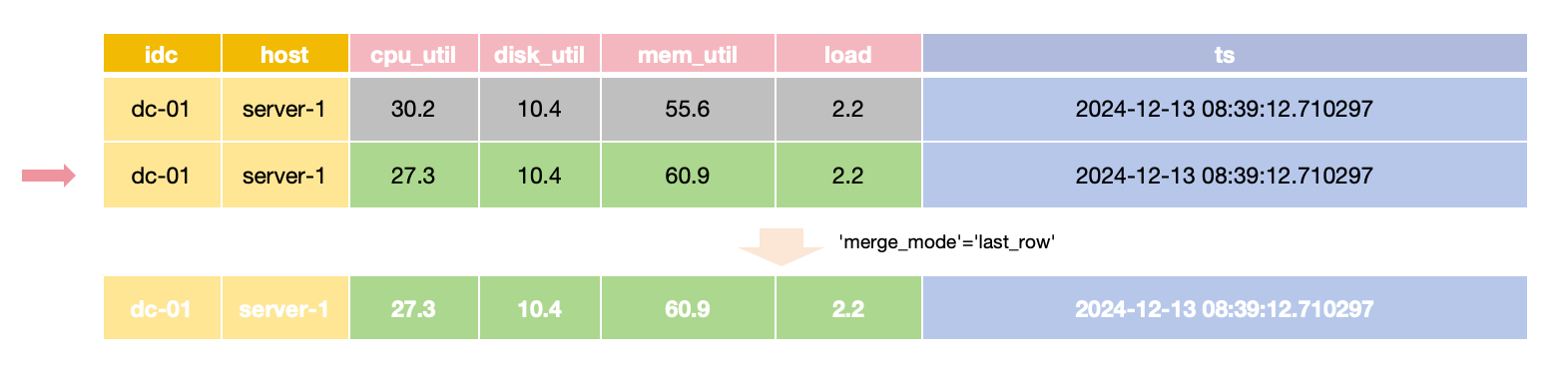
In `last_row` merge mode,
the latest row is returned for queries with the same primary key and time value,
requiring all Field values to be provided during updates.
For scenarios where only specific Field values need updating while others remain unchanged,
the `merge_mode` option can be set to `last_non_null`.
This mode retains the latest non-null value for each field during queries,
allowing updates to provide only the values that need to change.
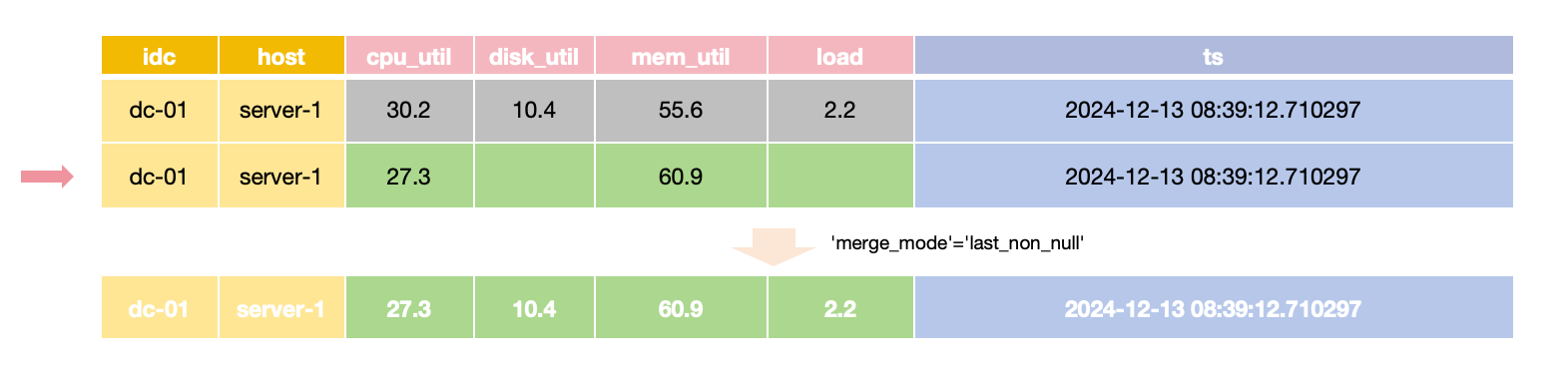
The `last_non_null` merge mode is the default for tables created automatically via the InfluxDB line protocol,
aligning with InfluxDB's update behavior.
The `last_row` merge mode doesn't have to check each individual field value so it is usually faster than the `last_non_null` mode.
Note that `merge_mode` cannot be set for Append-Only tables, as they do not perform merges.
### When to use append-only tables
If you don't need the following features, you can use append-only tables:
- Deduplication
- Deletion
GreptimeDB implements `DELETE` via deduplicating rows so append-only tables don't support deletion now.
Deduplication requires more computation and restricts the parallelism of ingestion and querying.
Using append-only tables usually has better query performance.
## Wide Table vs. Multiple Tables
In monitoring or IoT scenarios, multiple metrics are often collected simultaneously.
We recommend placing metrics collected simultaneously into a single table to improve read/write throughput and data compression efficiency.
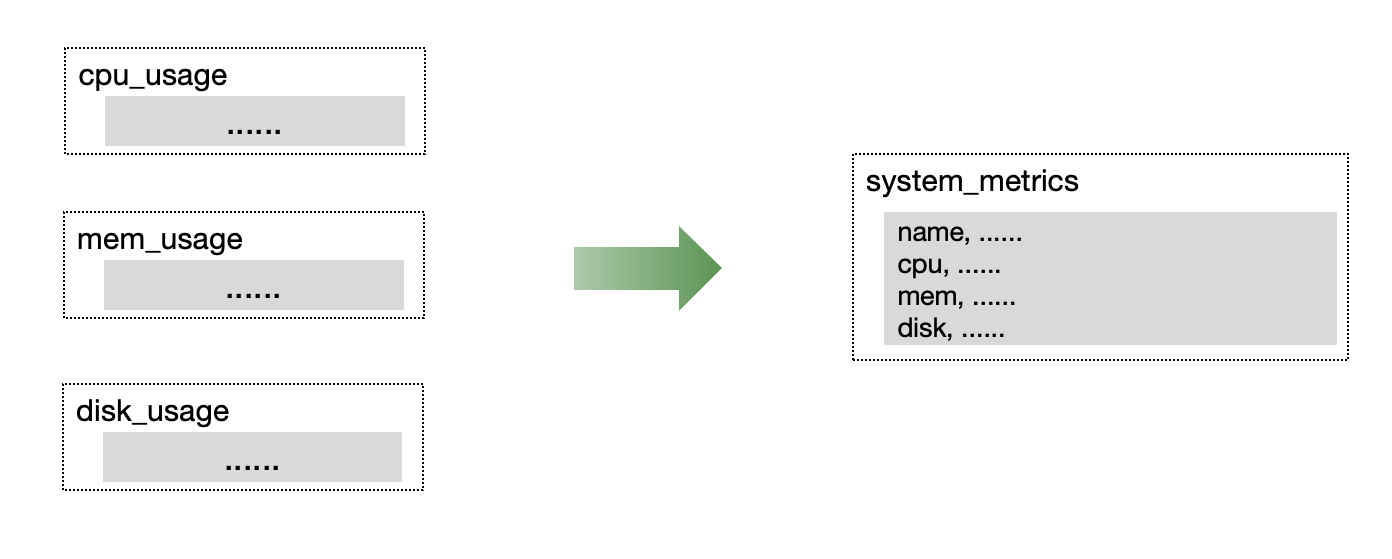
Although Prometheus uses single-value model for metrics, GreptimeDB's Prometheus Remote Storage protocol supports sharing a wide table for metrics at the underlying layer through the [Metric Engine](/contributor-guide/datanode/metric-engine.md).
## Distributed Tables
GreptimeDB supports partitioning data tables to distribute read/write hotspots and achieve horizontal scaling.
### Two misunderstandings about distributed tables
As a time-series database, GreptimeDB automatically partitions data based on the TIME INDEX column at the storage layer.
Therefore, it is unnecessary and not recommended for you to partition data by time
(e.g., one partition per day or one table per week).
Additionally, GreptimeDB is a columnar storage database,
so partitioning a table refers to horizontal partitioning by rows,
with each partition containing all columns.
### When to Partition and Determining the Number of Partitions
A table can utilize all the resources in the machine, especially during query.
Partitioning a table may not always improve the performance:
- A distributed query plan isn't always as efficient as a local query plan.
- Distributed query may introduce additional data transmission across the network.
There is no need to partition a table unless a single machine isn't enough to serve the table.
For example:
- There is not enough local disk space to store the data or to cache the data when using object stores.
- You need more CPU cores to improve the query performance or more memory for costly queries.
- The disk throughput becomes the bottleneck.
- The ingestion rate is larger than the throughput of a single node.
GreptimeDB releases a [benchmark report](https://github.com/GreptimeTeam/greptimedb/tree/v1.0.2/docs/benchmarks/tsbs) with each major version update,
detailing the ingestion throughput of a single partition.
Use this report alongside your target scenario to estimate if the write volume approaches the single partition's limit.
To estimate the total number of partitions,
consider the write throughput and reserve an additional 50% resource of CPU
to ensure query performance and stability. Adjust this ratio as necessary.
You can reserve more CPU cores if there are more queries.
### Partitioning Methods
GreptimeDB employs expressions to define partitioning rules.
For optimal performance,
select partition keys that are evenly distributed, stable, and align with query conditions.
Examples include:
- Partitioning by the prefix of a trace id.
- Partitioning by data center name.
- Partitioning by business name.
The partition key should closely match the query conditions.
For instance, if most queries target data from a specific data center,
using the data center name as a partition key is appropriate.
If the data distribution is not well understood, perform aggregate queries on existing data to gather relevant information.
For more details, refer to the [table partition guide](/user-guide/deployments-administration/manage-data/table-sharding.md#partition).
---
## Performance Tuning Tips
A GreptimeDB instance's default configuration may not fit all use cases. It's important to tune the database configurations and usage according to the scenario.
GreptimeDB provides various metrics to help monitor and troubleshoot performance issues. The official repository provides [Grafana dashboard templates](https://github.com/GreptimeTeam/greptimedb/tree/main/grafana) for both standalone and cluster modes.
## Query
### ANALYZE QUERY
GreptimeDB supports query analysis functionality.
Using the `EXPLAIN ANALYZE [VERBOSE] ` statement, you can view step-by-step query execution times.
### Metrics
The following metrics help diagnose query performance issues:
| Metric | Type | Description |
|---|---|---|
| greptime_mito_read_stage_elapsed_bucket | histogram | The elapsed time of different phases of a query in the storage engine. |
| greptime_mito_cache_bytes | gauge | Size of cached contents |
| greptime_mito_cache_hit | counter | Total count of cache hit |
| greptime_mito_cache_miss | counter | Total count of cache miss |
### Enlarging cache size
You can monitor the `greptime_mito_cache_bytes` and `greptime_mito_cache_miss` metrics to determine if you need to increase the cache size. The `type` label in these metrics indicates the type of cache.
If the `greptime_mito_cache_miss` metric is consistently high and increasing, or if the `greptime_mito_cache_bytes` metric reaches the cache capacity, you may need to adjust the cache size configurations of the storage engine.
Here is an example:
```toml
[[region_engine]]
[region_engine.mito]
# Cache size for the write cache. The `type` label value for this cache is `file`.
write_cache_size = "10G"
# Download files from object storage to fill the cache on write cache miss
enable_refill_cache_on_read = true
# Cache size for SST metadata. The `type` label value for this cache is `sst_meta`.
sst_meta_cache_size = "128MB"
# Cache size for vectors and arrow arrays. The `type` label value for this cache is `vector`.
vector_cache_size = "512MB"
# Cache size for pages of SST row groups. The `type` label value for this cache is `page`.
page_cache_size = "512MB"
# Cache size for time series selector (e.g. `last_value()`). The `type` label value for this cache is `selector_result`.
selector_result_cache_size = "512MB"
[region_engine.mito.index]
## The max capacity of the index staging directory.
staging_size = "10GB"
```
Some tips:
- 1/10 of disk space for the write cache at least. It's recommended to use a large write cache when using object storage.
- When using object storage, GreptimeDB automatically downloads files to fill the write cache on cache misses by default (`enable_refill_cache_on_read = true`). This improves query performance but may increase network traffic. Consider disabling this if you want to minimize network usage or storage costs.
- 1/4 of total memory for the `page_cache_size` at least if the memory usage is under 20%
- Double the cache size if the cache hit ratio is less than 50%
- If using full-text index, leave 1/10 of disk space for the `staging_size` at least
### Choosing the right SST format
GreptimeDB supports two [SST formats](/reference/sql/create.md#create-a-table-with-sst-format): `flat` and `primary_key`. Choosing the right one based on the cardinality of your primary key can significantly improve performance.
- **`flat` format (default)**: Optimized for high cardinality primary keys. If your primary key contains columns like `trace_id` or `uuid`, the `flat` format delivers better write and query performance. For tables with high cardinality primary keys, also consider using an [append-only table](/reference/sql/create.md#create-an-append-only-table) to further improve performance.
- **`primary_key` format**: May offer better performance when the primary key cardinality is not high.
See [Choosing the SST format](/user-guide/deployments-administration/performance-tuning/design-table.md#choosing-the-sst-format) for more details, including how to switch the format on existing tables.
### Using append-only table if possible
In general, append-only tables have a higher scan performance as the storage engine can skip merging and deduplication. What's more, the query engine can use statistics to speed up some queries if the table is append-only.
We recommend enabling the [append_mode](/reference/sql/create.md#create-an-append-only-table) for the table if it doesn't require deduplication or performance is prioritized over deduplication. For example, a log table should be append-only as log messages may have the same timestamp.
### Disable Write-Ahead-Log(WAL)
If you are consuming and writing to GreptimeDB from replayable data sources such as Kafka, you can further improve write throughput by disabling WAL.
Please note that when WAL is disabled, unflushed data to disk or object storage will not be recoverable and will need to be restored from the original data source, such as re-reading from Kafka or re-fetching logs.
Disable WAL by setting the table option `skip_wal='true'`:
```sql
CREATE TABLE logs(
message STRING,
ts TIMESTAMP TIME INDEX
) WITH (skip_wal = 'true');
```
## Ingestion
### Metrics
The following metrics help diagnose ingestion issues:
| Metric | Type | Description |
| -------------------------------------------- | --------- | ---------------------------------------------------------------------------------------- |
| greptime_mito_write_stage_elapsed_bucket | histogram | The elapsed time of different phases of processing a write request in the storage engine |
| greptime_mito_write_buffer_bytes | gauge | The current estimated bytes allocated for the write buffer (memtables). |
| greptime_mito_write_rows_total | counter | The number of rows written to the storage engine |
| greptime_mito_write_stall_total | gauge | The number of rows currently stalled due to high memory pressure |
| greptime_mito_write_reject_total | counter | The number of rows rejected due to high memory pressure |
| raft_engine_sync_log_duration_seconds_bucket | histogram | The elapsed time of flushing the WAL to the disk |
| greptime_mito_flush_elapsed | histogram | The elapsed time of flushing the SST files |
### Batching rows
Batching means sending multiple rows to the database over the same request. This can significantly improve ingestion throughput. A recommended starting point is 1000 rows per batch. You can enlarge the batch size if latency and resource usage are still acceptable.
### Writing by time window
Although GreptimeDB can handle out-of-order data, it still affects performance. GreptimeDB infers a time window size from ingested data and partitions the data into multiple time windows according to their timestamps. If the written rows are not within the same time window, GreptimeDB needs to split them, which affects write performance.
Generally, real-time data doesn't have the issues mentioned above as they always use the latest timestamp. If you need to import data with a long time range into the database, we recommend creating the table in advance and [specifying the compaction.twcs.time_window option](/reference/sql/create.md#create-a-table-with-custom-compaction-options).
## Schema
### Using multiple fields
While designing the schema, we recommend putting related metrics that can be collected together in the same table. This can also improve the write throughput and compression ratio.
For example, the following three tables collect the CPU usage metrics.
```sql
CREATE TABLE IF NOT EXISTS cpu_usage_user (
hostname STRING NULL,
usage_value BIGINT NULL,
ts TIMESTAMP(9) NOT NULL,
TIME INDEX (ts),
PRIMARY KEY (hostname)
);
CREATE TABLE IF NOT EXISTS cpu_usage_system (
hostname STRING NULL,
usage_value BIGINT NULL,
ts TIMESTAMP(9) NOT NULL,
TIME INDEX (ts),
PRIMARY KEY (hostname)
);
CREATE TABLE IF NOT EXISTS cpu_usage_idle (
hostname STRING NULL,
usage_value BIGINT NULL,
ts TIMESTAMP(9) NOT NULL,
TIME INDEX (ts),
PRIMARY KEY (hostname)
);
```
We can merge them into one table with three fields.
```sql
CREATE TABLE IF NOT EXISTS cpu (
hostname STRING NULL,
usage_user BIGINT NULL,
usage_system BIGINT NULL,
usage_idle BIGINT NULL,
ts TIMESTAMP(9) NOT NULL,
TIME INDEX (ts),
PRIMARY KEY (hostname)
);
```
---
## Run on Android Platforms
Since v0.4.0, GreptimeDB supports running on Android platforms with ARM64 CPU and Android API level >= 23.
## Install terminal emulator on Android
You can install [Termux](https://termux.dev/) from [GitHub release page](https://github.com/termux/termux-app/releases/latest).
## Download GreptimeDB Android binary.
```bash
VERSION=$(curl -sL \
-H "Accept: application/vnd.github+json" \
-H "X-GitHub-Api-Version: 2022-11-28" \
"https://api.github.com/repos/GreptimeTeam/greptimedb/releases/latest" | sed -n 's/.*"tag_name": "\([^"]*\)".*/\1/p')
curl -sOL "https://github.com/GreptimeTeam/greptimedb/releases/download/${VERSION}/greptime-android-arm64-${VERSION}.tar.gz"
tar zxvf ./greptime-android-arm64-${VERSION}.tar.gz
./greptime -V
```
If binary's downloaded correctly, the command is expected to print the version of downloaded binary.
## Create GreptimeDB configuration file
You can create a minimal configuration file that allows access from local network.
```bash
DATA_DIR="$(pwd)/greptimedb-data"
mkdir -p ${DATA_DIR}
cat < ./config.toml
[http]
addr = "0.0.0.0:4000"
[grpc]
bind_addr = "0.0.0.0:4001"
[mysql]
addr = "0.0.0.0:4002"
[storage]
data_home = "${DATA_DIR}"
type = "File"
EOF
```
## Start GreptimeDB from command line
```bash
./greptime --log-dir=$(pwd)/logs standalone start -c ./config.toml
```
## Connect to GreptimeDB running on Android
> You can find the IP address of your Android device from system settings or `ifconfig`.
You can now connect to the GreptimeDB instance running on Android from another device with MySQL client installed.
```bash
mysql -h -P 4002
```
And play like on any other platforms!
```
Welcome to the MySQL monitor. Commands end with ; or \g.
Your MySQL connection id is 8
Server version: 5.1.10-alpha-msql-proxy Greptime
Copyright (c) 2000, 2023, Oracle and/or its affiliates.
Oracle is a registered trademark of Oracle Corporation and/or its
affiliates. Other names may be trademarks of their respective
owners.
Type 'help;' or '\h' for help. Type '\c' to clear the current input statement.
mysql> CREATE TABLE monitor (env STRING, host STRING, ts TIMESTAMP, cpu DOUBLE DEFAULT 0, memory DOUBLE, TIME INDEX (ts), PRIMARY KEY(env,host));
Query OK, 0 rows affected (0.14 sec)
mysql> INSERT INTO monitor(ts, env, host, cpu, memory) VALUES
-> (1655276557000,'prod', 'host1', 66.6, 1024),
-> (1655276557000,'prod', 'host2', 66.6, 1024),
-> (1655276557000,'prod', 'host3', 66.6, 1024),
-> (1655276558000,'prod', 'host1', 77.7, 2048),
-> (1655276558000,'prod', 'host2', 77.7, 2048),
-> (1655276558000,'test', 'host3', 77.7, 2048),
-> (1655276559000,'test', 'host1', 88.8, 4096),
-> (1655276559000,'test', 'host2', 88.8, 4096),
-> (1655276559000,'test', 'host3', 88.8, 4096);
Query OK, 9 rows affected (0.14 sec)
mysql>
mysql> select * from monitor where env='test' and host='host3';
+------+-------+---------------------+------+--------+
| env | host | ts | cpu | memory |
+------+-------+---------------------+------+--------+
| test | host3 | 2022-06-15 15:02:38 | 77.7 | 2048 |
| test | host3 | 2022-06-15 15:02:39 | 88.8 | 4096 |
+------+-------+---------------------+------+--------+
2 rows in set (0.20 sec)
```
---
## Troubleshooting
When encountering errors or performance issues,
you can understand GreptimeDB's status through metrics and logs.
This information can also help further investigate the root causes of problems.
The following lists troubleshooting methods for some common abnormal situations.
For cases where the cause cannot be easily identified,
providing metrics and logs to the official team can also improve the efficiency of official troubleshooting.
## Checking CPU and Memory Load
You can directly view the CPU and Memory load of corresponding components from the Dashboard.
CPU is displayed in millicores, while Memory shows the current process RSS.
You need to pay attention to whether the corresponding CPU and Memory load exceeds the Pod's Limit.
If CPU has reached the Pod's Limit,
throttling will be triggered, and clients will experience slower request processing.
If Memory reaches over 70% of the Limit, it may result in OOM (Out of Memory).
## Flow Creation Failure
When flow creation fails,
one common scenario is that flownode is not deployed.
You can check:
- Whether flownode is deployed in the cluster
- Whether the flownode status in the cluster is READY
If flownode is already deployed,
you can further investigate by examining metasrv and flownode logs,
or check whether the flow node was successfully created through internal tables:
```sql
select * from information_schema.cluster_info;
```
## Object Storage Configuration Issues
When object storage is misconfigured,
GreptimeDB will encounter exceptions when accessing object storage.
If GreptimeDB hasn't stored any data,
it generally doesn't need to access object storage,
so errors might not be observable immediately after deployment.
Once you create a table or start writing data to GreptimeDB through write protocols, you can observe request errors.
Typically, DB error messages will include object storage error details.
You can find specific object storage error information through DB error logs.
Some common error causes include:
- Incorrect Access Key or Secret Access Key
- Improper object storage permission configuration
- If using Tencent Cloud COS's S3-compatible API, since Tencent Cloud has [disabled path-style domains](https://cloud.tencent.com/document/product/436/102489), you need to set `enable_virtual_host_style = true` in GreptimeDB's S3 configuration
For S3 as an example, GreptimeDB requires the following permissions:
```txt
"s3:PutObject",
"s3:ListBucket",
"s3:GetObject",
"s3:DeleteObject"
```
## Low Write Throughput
You can observe write throughput through the Ingestion-related panels in the dashboard:
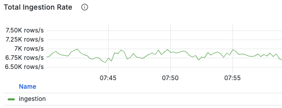
If write throughput is lower than expected load
it might be due to high write latency causing DB backlog.
The dashboard provides panels in the `Frontend Requests` area to observe request latency:
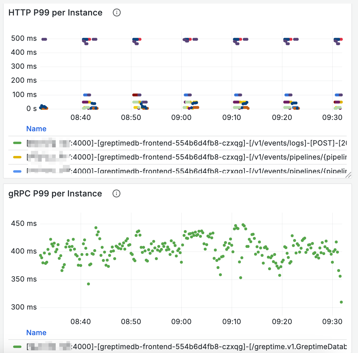
You can check if any nodes are experiencing stall through the `Write Stall` panel in the `Mito Engine` area (stall values remaining above 0 for extended periods).
If so, it indicates that node writes have encountered bottlenecks.
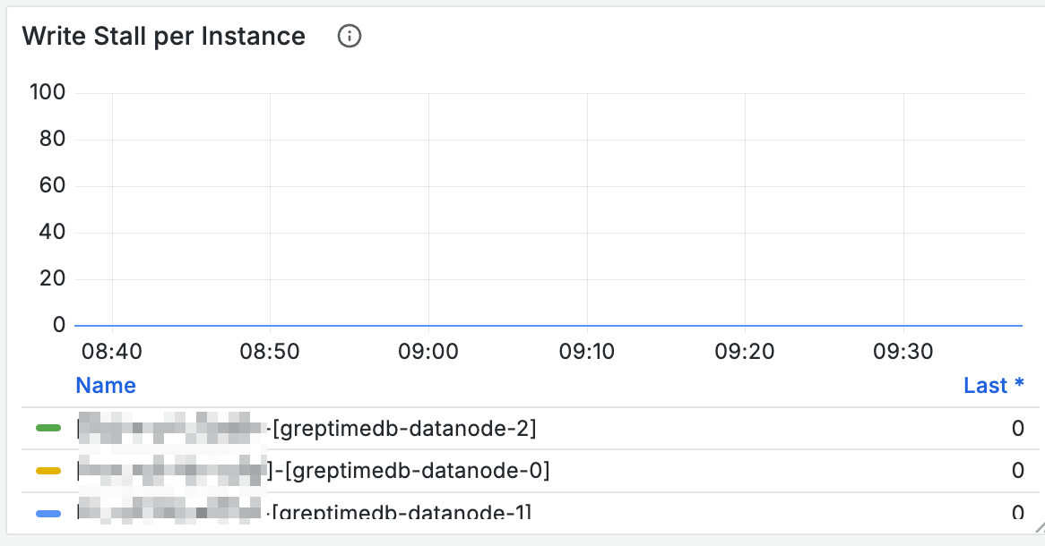
By observing the `Write Buffer` panel, you can also monitor size changes in buffers used for writing. If buffers fill up quickly, consider proportionally increasing `global_write_buffer_size` and `global_write_buffer_reject_size`:
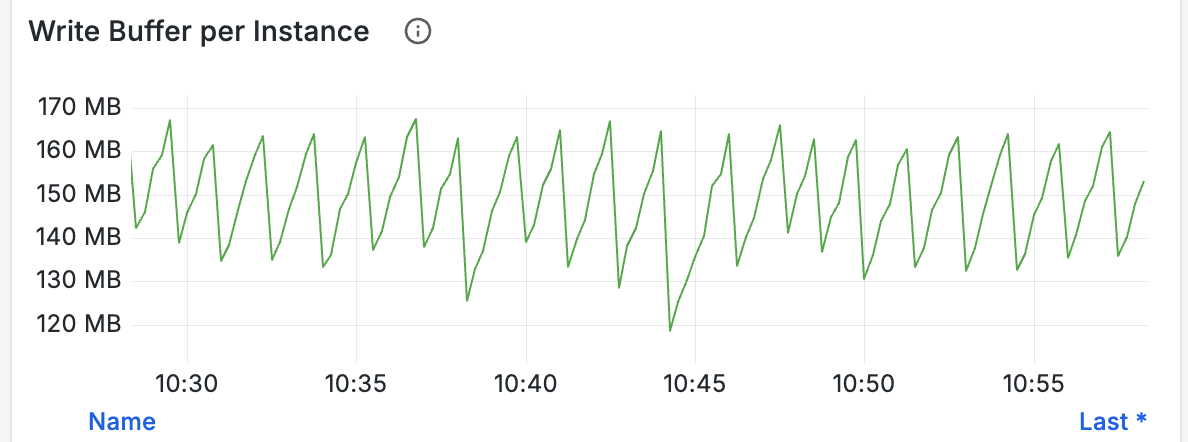
The Write Stage panel shows which stages have high write latency:
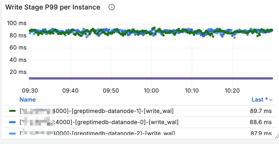
You can check background task status through Compaction/Flush related panels:
- Whether frequent flush operations occur; if so, consider proportionally increasing `global_write_buffer_size` and `global_write_buffer_reject_size`
- Whether there are long-running compaction and flush operations; if so, writes might be affected by these background tasks
Additionally, logs related to `flush memtables` can show the latency of individual flush operations.
## High Memory Consumption During Writes
During DB write operations,
the total size of all memtables is estimated.
You can view memtable memory usage through the `Write Buffer` panel.
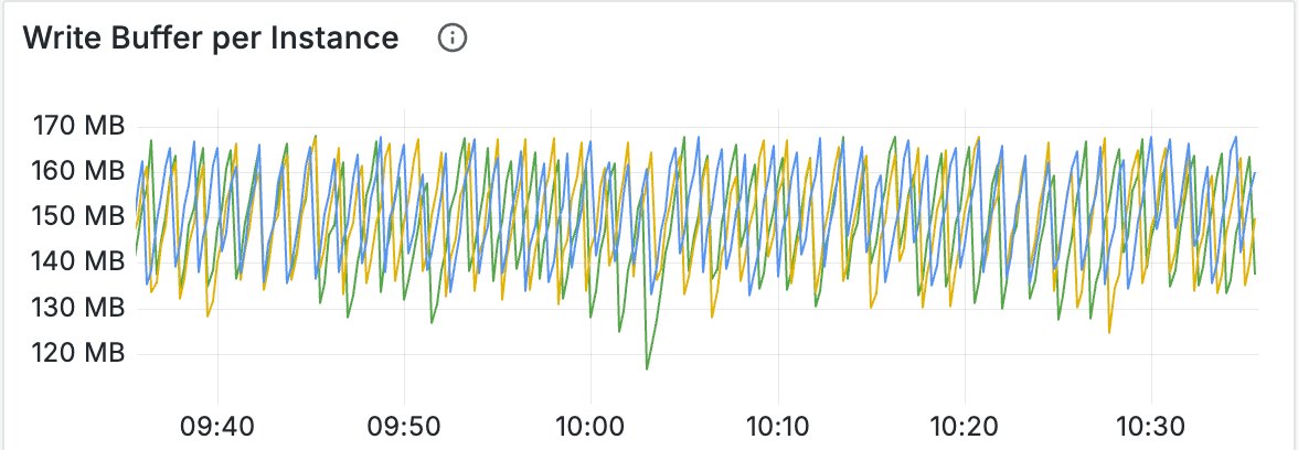
Note that these values might be smaller than the actual allocated memory.
If you notice that DB memory grows too quickly during writes,
or if writes frequently encounter OOM situations,
this might be related to unreasonable table schema design.
A common cause is improper Primary Key design.
If there are too many primary keys,
it will consume excessive memory during writes,
potentially causing database memory usage to become too high.
In such cases, `Write Buffer` often remains at high levels.
Increasing write buffer size generally won't improve this issue;
you need to reduce the number of primary key columns or remove high-cardinality primary key columns.
## High Query Latency
If query latency is high,
you can add `EXPLAIN ANALYZE` or `EXPLAIN ANALYZE VERBOSE` before the query and re-execute it.
The query results will include execution time for each stage to assist in troubleshooting.
Additionally, the `Read Stage` panel can help understand query latency across different stages:
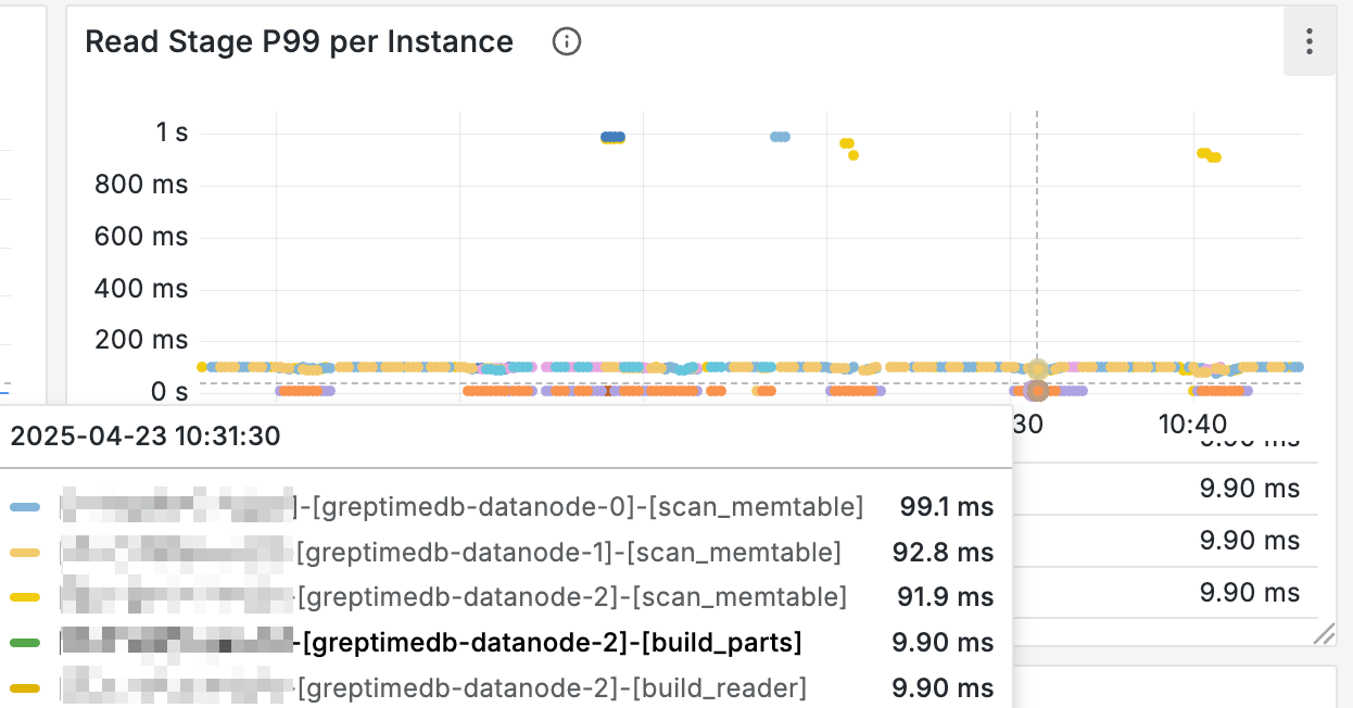
## Cache Full
To understand the size of various caches,
you can check the used size of different caches on nodes through the `Cached Bytes` panel:
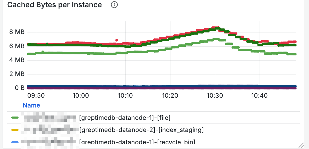
For nodes with high query latency,
you can also determine if caches are full by checking cache sizes.
## Object Storage Latency
You can view object storage operation latency through panels in the `OpenDAL` area of the dashboard.
For example, the following panel shows response latency for object storage write operations:
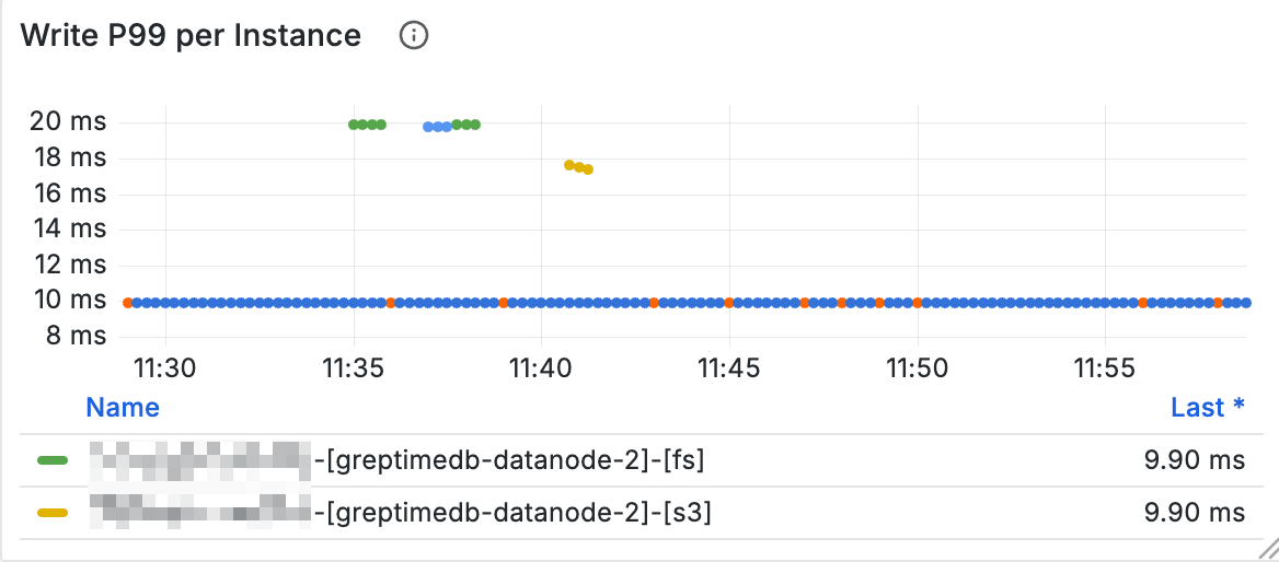
If you suspect object storage operations are experiencing jitter,
you can observe the related panels.
---
## Upgrade
## Overview
This guide provides upgrade instructions for GreptimeDB, including compatibility information and breaking changes for each version. Before upgrading, ensure you review the relevant breaking changes for your upgrade path.
For complete version history and feature additions, see the [Release Notes](/release-notes/).
## Upgrade Paths to v1.0
### From v0.16 to v1.0
If you are currently running v0.16, you can upgrade directly to v1.0. See [Upgrading from v0.16 to v1.0](#upgrading-from-v016-to-v10) for all relevant breaking changes.
### From v0.17 to v1.0
If you are currently running v0.17, you can upgrade directly to v1.0. See [Upgrading from v0.17 to v1.0](#upgrading-from-v017-to-v10) for breaking changes.
### From Earlier Versions
**Important:** This guide only covers upgrades from v0.16 and later versions.
If you are running a version earlier than v0.16, you must first upgrade to v0.16 by following the upgrade documentation for your current version. Once you have successfully upgraded to v0.16, you can then use this guide to upgrade to v1.0.
## Breaking Changes by Version
### Upgrading from v0.17 to v1.0
#### Jaeger HTTP Header Removal
**Impact:** HTTP header deprecation
The HTTP header `x-greptime-jaeger-time-range-for-operations` has been deprecated and removed.
**Action Required:**
- If you configured this header in your Jaeger data source or proxy, remove it from your configuration
- The header will no longer have any effect
#### Metric Engine Default Sparse Primary Key Encoding
**Impact:** Default configuration change with performance improvements
Metric Engine now enables **sparse primary key encoding** by default to improve storage efficiency and query performance for metric scenarios.
**Configuration Changes:**
- **NEW default:** `sparse_primary_key_encoding = true`
- **DEPRECATED:** `experimental_sparse_primary_key_encoding` (use `sparse_primary_key_encoding` instead)
**Action Required:**
- This change does not cause data format compatibility issues
- All metric tables will automatically use sparse encoding by default
- If you want to continue using the old encoding method, explicitly set:
```toml
[metric_engine]
sparse_primary_key_encoding = false
```
#### `greptime_identity` Pipeline JSON Behavior Change
**Impact:** JSON processing logic change
The JSON processing logic in `greptime_identity` pipeline has changed significantly:
**New Behavior:**
- Nested JSON objects are automatically flattened into separate columns using dot notation (e.g., `object.a`, `object.b`)
- Arrays are stored as JSON strings instead of JSON objects
- The `flatten_json_object` parameter has been removed
- A new `max_nested_levels` parameter controls flattening depth (default: 10 levels)
- When the depth limit is exceeded, remaining nested structures are serialized as JSON strings
**Action Required:**
1. Review your pipeline configurations that use `greptime_identity`
2. Remove any usage of the deprecated `flatten_json_object` parameter
3. Adjust queries that reference nested JSON fields to use the new dot notation
4. If you have deeply nested JSON (>10 levels), consider setting `max_nested_levels` appropriately
**Example:**
Before (v0.17):
```json
{ "user": { "name": "Alice", "age": 30 } }
```
Stored as a single JSON column.
After (v1.0):
```
user.name = "Alice"
user.age = 30
```
Stored as separate columns.
#### Metric Engine TSID Generation Algorithm Change
**Impact:** Time Series ID generation optimization with query implications
The TSID (Time Series ID) generation algorithm has been optimized by replacing `mur3::Hasher128` with the higher-performance `fxhash::FxHasher`, including a fast-path for series without NULL labels.
**Performance Improvements:**
- Regular scenarios: 5-6x faster
- Scenarios with NULL labels: ~2.5x faster
**Breaking Change Impact:**
This is a **breaking change** that affects time series identification:
- **Before upgrade (time < t):** Data uses the old algorithm to generate TSIDs
- **After upgrade (time > t):** Data uses the new algorithm to generate TSIDs
**Query Behavior:**
- Queries with time ranges that **span the upgrade time `t`** may experience slight discrepancies in time series matching near time `t`
- Queries with time ranges that **do not include `t`** are not affected
**Action Required:**
Choose one of the following upgrade strategies:
1. **Direct Upgrade (Recommended for most users):**
- Accept minor query discrepancies near the upgrade time
- Suitable if approximate results near the upgrade time are acceptable
2. **Export-Upgrade-Import (For zero tolerance):**
- If you cannot accept any discrepancies, use this fully compatible upgrade method:
1. Export all data before upgrading
2. Upgrade to v1.0
3. Import data back into the new version
- Refer to [Backup & Restore Documentation](/user-guide/deployments-administration/disaster-recovery/back-up-&-restore-data/)
### Upgrading from v0.16 to v1.0
If you are upgrading from v0.16, you need to review:
1. **All breaking changes from v0.17 to v1.0** (listed above)
2. **v0.17.0 breaking changes** (listed below)
This ensures you're aware of all changes that occurred between v0.16 and v1.0.
### v0.17.0 Breaking Changes
#### Ordered-Set Aggregate Functions
**Impact:** SQL syntax change
Ordered-set aggregate functions now require a `WITHIN GROUP (ORDER BY …)` clause.
**Before:**
```sql
SELECT approx_percentile_cont(latency, 0.95) FROM metrics;
```
**After:**
```sql
SELECT approx_percentile_cont(0.95) WITHIN GROUP (ORDER BY latency) FROM metrics;
```
**Action Required:** Update all queries using ordered-set aggregate functions (`approx_percentile_cont`, `approx_percentile_cont_weight`, etc.) to include the `WITHIN GROUP (ORDER BY …)` clause.
#### MySQL Protocol Comment Styling
**Impact:** Comment syntax strictness
Incorrect comment styling is no longer allowed in MySQL protocol. Comments must start with `--` instead of `---`.
**Before:**
```sql
--- This is a comment
SELECT * FROM table;
```
**After:**
```sql
-- This is a comment
SELECT * FROM table;
```
**Action Required:** Update any SQL scripts or queries that use `---` style comments to use the standard `--` format.
## Additional v1.0 Changes (Non-Breaking)
### v1.0.0-beta.3
#### Cache Configuration Improvements
The cache architecture has been refactored for better performance:
**New Configuration:**
- `region_engine.mito.manifest_cache_size` (default: 256MB) - specialized manifest file cache
**Removed Configuration:**
- `storage.cache_path`
- `storage.enable_read_cache`
- `storage.cache_capacity`
**Action Required:** Update your configuration files to use the new `manifest_cache_size` setting and remove the deprecated storage cache options.
### v1.0.0-beta.2
#### Improved Database Compatibility
- Numeric type aliases aligned with PostgreSQL and MySQL standards
- Better PostgreSQL extended query support
- Improved MySQL binary protocol handling
**Action Required:** Test your applications to ensure compatibility with the improved behavior.
## Minimizing Business Impact During Upgrade
Before upgrading GreptimeDB, it is essential to perform a comprehensive backup of your data to safeguard against potential data loss. This backup acts as a safety measure in the event of any issues during the upgrade process.
### Best Practices
#### Rolling Upgrade
Utilize [rolling upgrades](https://kubernetes.io/docs/tutorials/kubernetes-basics/update/update-intro/) on Kubernetes to update GreptimeDB instances incrementally. This approach replaces old instances with new ones while maintaining service availability and minimizing downtime.
#### Automatic Retries
Configure client applications to enable automatic retries with exponential backoff. This helps handle temporary service interruptions gracefully.
#### Temporary Pause of Write Operations
For applications that can tolerate brief maintenance windows, consider pausing write operations during the upgrade to ensure data consistency.
#### Double Writing
Implement double writing to both the old and new versions of GreptimeDB, then switch to the new version once you have verified that it is functioning correctly. This allows you to verify data consistency and gradually redirect read traffic to the upgraded version.
## Upgrade Checklist
Before upgrading to v1.0, complete the following checklist:
### Pre-Upgrade
- [ ] Review all breaking changes relevant to your upgrade path
- [ ] **Backup all data and configurations**
- [ ] Identify queries using ordered-set aggregate functions (if upgrading from v0.16 or earlier)
- [ ] Identify pipelines using `greptime_identity` with JSON data
- [ ] Check for usage of deprecated Jaeger HTTP header (if upgrading from v0.17 or earlier)
- [ ] Review metric tables if using Metric Engine
### Configuration Updates
- [ ] Update configuration files (remove deprecated cache settings)
- [ ] Update metric engine configuration if needed (`sparse_primary_key_encoding`)
- [ ] Update pipeline configurations (remove `flatten_json_object`, add `max_nested_levels` if needed)
### Code Updates
- [ ] Update SQL queries with ordered-set aggregates to use `WITHIN GROUP (ORDER BY ...)`
- [ ] Update SQL scripts using `---` comments to use `--`
- [ ] Update queries that access nested JSON fields to use dot notation
- [ ] Remove Jaeger header configuration if present
### Testing & Deployment
- [ ] Test the upgrade in a non-production environment
- [ ] Verify query results, especially for:
- Ordered-set aggregate functions
- Nested JSON data access
- Metric queries (if affected by TSID change)
- [ ] Plan for rolling upgrade or maintenance window
- [ ] Prepare rollback plan in case of issues
- [ ] Monitor system behavior after upgrade
### Special Considerations for Metric Engine Users
If you cannot accept query discrepancies near the upgrade time due to TSID algorithm change:
- [ ] Plan for export-upgrade-import process
- [ ] Allocate sufficient time for data export and import
- [ ] Refer to [Backup & Restore Documentation](/user-guide/deployments-administration/disaster-recovery/back-up-&-restore-data/)
---
## Local WAL
This section describes how to configure the local WAL for GreptimeDB Datanode component.
```toml
[wal]
provider = "raft_engine"
file_size = "128MB"
purge_threshold = "1GB"
purge_interval = "1m"
read_batch_size = 128
sync_write = false
```
## Options
If you are using Helm Chart to deploy GreptimeDB, you can refer to [Common Helm Chart Configurations](/user-guide/deployments-administration/deploy-on-kubernetes/common-helm-chart-configurations.md) to learn how to configure the Datanode by injecting configuration files.
| Configuration Option | Description | Default Value |
| -------------------- | -------------------------------------------------------------------------------------------------------------------- | ----------------- |
| `provider` | The provider of the WAL. Options: `raft_engine` (local file system storage), `kafka` (remote WAL storage in Kafka), or `noop` (no-op WAL provider) | `"raft_engine"` |
| `dir` | The directory where to write logs | `{data_home}/wal` |
| `file_size` | The size of single WAL log file | `128MB` |
| `purge_threshold` | The threshold of the WAL size to trigger purging | `1GB` |
| `purge_interval` | The interval to trigger purging | `1m` |
| `read_batch_size` | The read batch size | `128` |
| `sync_write` | Whether to call fsync when writing every log | `false` |
## Best practices
### Using a separate High-Performance Volume for WAL
It is beneficial to configure a separate volume for the WAL (Write-Ahead Log) directory when deploying GreptimeDB. This setup allows you to:
- Leverage a high-performance disk—either a dedicated physical volume or one provisioned via a custom `StorageClass`.
- Isolate WAL I/O from cache file access, reducing I/O contention and enhancing overall system performance.
If you are using Helm Chart to deploy GreptimeDB, you can refer to [Common Helm Chart Configurations](/user-guide/deployments-administration/deploy-on-kubernetes/common-helm-chart-configurations.md) to learn how to configure a dedicated WAL volume.
---
## Noop WAL
Noop WAL is a special WAL provider for emergency situations when the configured WAL provider becomes temporarily unavailable. It does not store any WAL data.
## Availability
Noop WAL is **only available in cluster mode**, not in standalone mode.
## Use Cases
- **Temporary WAL Unavailability**: When the WAL provider (e.g., Kafka) is temporarily unavailable, switch the Datanode to Noop WAL to keep the cluster running.
- **Testing and Development**: Useful for testing scenarios where WAL persistence is not required.
## Data Loss Warning
**When using Noop WAL, all unflushed data will be lost when the Datanode is shutdown or restarted.** Only use this provider temporarily when the normal WAL provider is unavailable. Not recommended for production use except in emergency situations.
## Configuration
To configure Noop WAL for a Datanode:
```toml
[wal]
provider = "noop"
```
In a GreptimeDB cluster, WAL configuration has two parts:
- **Metasrv** - Generates WAL metadata for new regions. Should be set to `raft_engine` or `kafka`.
- **Datanode** - Reads and writes WAL data. Configure as `noop` when the WAL provider is unavailable.
Note: Noop WAL can only be configured on Datanode, not on Metasrv. When using Noop WAL on Datanode, Metasrv continues using its configured WAL provider.
## Best Practices
- Flush regions regularly using `admin flush_table()` or `admin flush_region()` to minimize data loss.
- Switch back to the normal WAL provider as soon as it becomes available.
---
## GreptimeDB WAL Overview
# Overview
The [Write-Ahead Logging](/contributor-guide/datanode/wal.md#introduction)(WAL) is a crucial component in GreptimeDB that persistently records every data modification to ensure no memory-cached data loss. GreptimeDB provides three WAL storage options:
- **Local WAL**: Uses an embedded storage engine([raft-engine](https://github.com/tikv/raft-engine)) within the [Datanode](/user-guide/concepts/why-greptimedb.md).
- **Remote WAL**: Uses [Apache Kafka](https://kafka.apache.org/) as the external(remote) WAL storage component.
- **Noop WAL**: A no-op WAL provider for emergency situations when WAL becomes unavailable. Does not store any data.
## Local WAL
### Advantages
- **Low latency**: The local WAL is stored within the same process as the Datanode, eliminating network overhead and providing low write latency.
- **Easy to deploy**: Since the WAL is co-located with the Datanode, no additional components are required, simplifying deployment and operations.
- **Zero RPO**: When deploying GreptimeDB in the cloud, you can configure persistent storage for WAL data using cloud storage services such as AWS EBS or GCP Persistent Disk. This ensures zero [Recovery Point Objective](https://en.wikipedia.org/wiki/Disaster_recovery#Recovery_Point_Objective) (RPO), meaning no data loss, even in the event of system failure.
### Disadvantages
- **High RTO**: Because the WAL resides on the same node as the Datanode, the [Recovery Time Objective](https://en.wikipedia.org/wiki/Disaster_recovery#Recovery_Time_Objective) (RTO) is relatively high. After a Datanode restarts, it must replay the WAL to restore the latest data, during which time the node remains unavailable.
- **Single-Point Access Limitation**: The local WAL is tightly coupled with the Datanode process and only supports a single consumer, which limits features such as region hot standby and [Region Migration](/user-guide/deployments-administration/manage-data/region-migration.md).
## Remote WAL
### Advantages
- **Low RTO**: By decoupling WAL from the Datanode, [Recovery Time Objective](https://en.wikipedia.org/wiki/Disaster_recovery#Recovery_Time_Objective) (RTO) is minimized. If a Datanode crashes, the Metasrv can quickly trigger a [Region Failover](/user-guide/deployments-administration/manage-data/region-failover.md) to migrate affected regions to healthy nodes—without the need to replay WAL locally.
- **Multi-Consumer Subscriptions**: Remote WAL supports multiple consumers subscribing to WAL logs simultaneously, enabling features such as region hot standby and [Region Migration](/user-guide/deployments-administration/manage-data/region-migration.md), thereby enhancing system availability and flexibility.
### Disadvantages
- **External dependencies**: Remote WAL relies on an external Kafka cluster, which increases the complexity of deployment, operation, and maintenance.
- **Network overhead**: Since WAL data needs to be transmitted over the network, careful planning of cluster network bandwidth is required to ensure low latency and high throughput, especially under write-heavy workloads.
## Noop WAL
Noop WAL is a special WAL provider for emergency situations when the configured WAL provider becomes temporarily unavailable. It does not store any WAL data and is only available in cluster mode.
For detailed configuration, see the [Noop WAL](/user-guide/deployments-administration/wal/noop-wal.md) page.
## Next steps
- To configure the Local WAL storage, please refer to [Local WAL](/user-guide/deployments-administration/wal/local-wal.md).
- To learn more about the Remote WAL, please refer to [Remote WAL](/user-guide/deployments-administration/wal/remote-wal/configuration.md).
- To learn more about the Noop WAL, please refer to [Noop WAL](/user-guide/deployments-administration/wal/noop-wal.md).
---
## GreptimeDB Remote WAL Configuration
# Configuration
The configuration of Remote WAL contains two parts:
- Metasrv Configuration
- Datanode Configuration
If you are using Helm Chart to deploy GreptimeDB, you can refer to [Common Helm Chart Configurations](/user-guide/deployments-administration/deploy-on-kubernetes/common-helm-chart-configurations.md) to learn how to configure Remote WAL.
## Metasrv Configuration
On the Metasrv side, Remote WAL is primarily responsible for managing Kafka topics and periodically pruning stale WAL data.
```toml
[wal]
provider = "kafka"
broker_endpoints = ["kafka.kafka-cluster.svc.cluster.local:9092"]
# WAL data pruning options
auto_prune_interval = "30m"
auto_prune_parallelism = 10
flush_trigger_size = "512MB"
checkpoint_trigger_size = "128MB"
# Topic creation options
auto_create_topics = true
num_topics = 64
replication_factor = 1
topic_name_prefix = "greptimedb_wal_topic"
create_topic_timeout = "30s"
```
### Options
| Configuration Option | Description |
|----------------------------|--------------------------------------------------------------------------------------------------------------------------------------------------------------------------------------------------------------------------------------------------------------------------------------------------------------------------------------------------------------------------------------------------------------------------------------------------------------------------------------------------|
| `provider` | The WAL provider to use. Set to `"kafka"` to enable Remote WAL with Kafka. |
| `broker_endpoints` | List of Kafka broker addresses to connect to. Example: `["kafka.kafka-cluster.svc:9092"]`. |
| `auto_prune_interval` | How often to automatically prune (delete) stale WAL data. Specify as a duration string (e.g., `"30m"`). Set to `"0s"` to disable automatic pruning. |
| `auto_prune_parallelism` | Maximum number of concurrent pruning tasks. Increasing this value may speed up pruning but will use more resources. |
| `auto_create_topics` | If `true`, Metasrv will automatically create required Kafka topics. If `false`, you must manually create all topics before starting Metasrv. |
| `num_topics` | Number of Kafka topics to use for WAL storage. More topics can improve scalability and performance. |
| `replication_factor` | Replication factor for Kafka topics. Determines how many Kafka brokers will store copies of each topic's data. |
| `topic_name_prefix` | Prefix for Kafka topic names. WAL topics will be named as `{topic_name_prefix}_{index}` (e.g., `greptimedb_wal_topic_0`). The prefix must match the regex `[a-zA-Z_:-][a-zA-Z0-9_:\-\.@#]*`. |
| `flush_trigger_size` | Estimated size threshold (e.g., `"512MB"`) for triggering a flush operation in a region. Calculated as `(latest_entry_id - flushed_entry_id) * avg_record_size`. When this value exceeds `flush_trigger_size`, MetaSrv initiates a flush. Set to `"0"` to let the system automatically determine the flush trigger size. This also controls the maximum replay size from a topic during region replay; using a smaller value can help reduce region replay time during Datanode startup. |
| `checkpoint_trigger_size` | Estimated size threshold (e.g., `"128MB"`) for triggering a checkpoint operation in a region. Calculated as `(latest_entry_id - last_checkpoint_entry_id) * avg_record_size`. When this value exceeds `checkpoint_trigger_size`, MetaSrv initiates a checkpoint. Set to `"0"` to let the system automatically determine the checkpoint trigger size. Using a smaller value can help reduce region replay time during Datanode startup. |
| `create_topic_timeout` | The timeout for creating a Kafka topic. Default is `"30s"`. |
#### Topic Setup and Kafka Permissions
To ensure Remote WAL works correctly with Kafka, please check the following:
- If `auto_create_topics = false`:
- All required topics must be created manually **before** starting Metasrv.
- Topic names must follow the pattern `{topic_name_prefix}_{index}` where `index` ranges from `0` to `{num_topics - 1}`. For example, with the default prefix `greptimedb_wal_topic` and `num_topics = 64`, you need to create topics from `greptimedb_wal_topic_0` to `greptimedb_wal_topic_63`.
- Topics must be configured to support **LZ4 compression**.
- The Kafka user must have the following permissions:
- **Append** records to WAL topics (requires LZ4 compression support).
- **Read** records from WAL topics (requires LZ4 compression support).
- **Delete** records from WAL topics.
- **Create** topics (only required if `auto_create_topics = true`).
## Datanode Configuration
The Datanode side is mainly used to write the data to the Kafka topics and read the data from the Kafka topics.
```toml
[wal]
provider = "kafka"
broker_endpoints = ["kafka.kafka-cluster.svc:9092"]
max_batch_bytes = "1MB"
overwrite_entry_start_id = true
connect_timeout = "3s"
timeout = "3s"
```
### Options
| Configuration Option | Description |
| -------------------------- | ----------------------------------------------------------------------------------------------------------------------------- |
| `provider` | Set to "kafka" to enable Remote WAL via Kafka. |
| `broker_endpoints` | List of Kafka broker addresses. |
| `max_batch_bytes` | Maximum size for each Kafka producer batch. |
| `overwrite_entry_start_id` | If true, the Datanode will skip over missing entries during WAL replay. Prevents out-of-range errors, but may hide data loss. |
| `connect_timeout` | The connect timeout for Kafka client. Default is `"3s"`. |
| `timeout` | The timeout for Kafka client operations. Default is `"3s"`. |
#### Required Settings and Limitations
:::warning IMPORTANT: Kafka Retention Policy Configuration
Please configure Kafka retention policy very carefully to avoid data loss. GreptimeDB will automatically recycle unneeded WAL data, so in most cases you don't need to set the retention policy. However, if you do set it, please ensure the following:
- **Size-based retention**: Typically not needed, as the database manages its own data lifecycle
- **Time-based retention**: If you choose to set this, ensure it's **significantly greater than the auto-flush-interval** to prevent premature data deletion
Improper retention settings can lead to data loss if WAL data is deleted before GreptimeDB has processed it.
:::
- If you set `overwrite_entry_start_id = true`:
- Ensure that `auto_prune_interval` is enabled in Metasrv to allow automatic WAL pruning.
- Kafka topics **must not use size-based retention policies**.
- If time-based retention is enabled, the retention period should be set to a value significantly greater than auto-flush-interval, preferably at least 2 times its value.
- Ensure the Kafka user used by Datanode has the following permissions:
- **Append** records to WAL topics (requires LZ4 compression support).
- **Read** records from WAL topics (requires LZ4 compression support).
- Ensure that `max_batch_bytes` does not exceed Kafka’s maximum message size (typically 1MB by default).
## Kafka Authentication Configuration
Kafka authentication settings apply to both Metasrv and Datanode under the `[wal]` section.
### SASL
Kafka supports several SASL mechanisms: `PLAIN`, `SCRAM-SHA-256`, and `SCRAM-SHA-512`.
```toml
[wal]
broker_endpoints = ["kafka.kafka-cluster.svc.cluster.local:9092"]
[wal.sasl]
type = "SCRAM-SHA-512"
username = "user"
password = "secret"
```
### TLS
You can enable TLS encryption for Kafka connections by configuring the `[wal.tls]` section. There are three common modes:
#### Using System CA Certificate
To use system-wide trusted CAs, enable TLS without providing any certificate paths:
```toml
[wal]
broker_endpoints = ["kafka.kafka-cluster.svc.cluster.local:9092"]
[wal.tls]
```
#### Using Custom CA Certificate
If your Kafka cluster uses a private CA, specify the server CA certificate explicitly:
```toml
[wal]
broker_endpoints = ["kafka.kafka-cluster.svc.cluster.local:9092"]
[wal.tls]
server_ca_cert_path = "/path/to/server.crt"
```
#### Using Mutual TLS (mTLS)
To enable mutual authentication, provide both the client certificate and private key along with the server CA:
```toml
[wal]
broker_endpoints = ["kafka.kafka-cluster.svc.cluster.local:9092"]
[wal.tls]
server_ca_cert_path = "/path/to/server_cert"
client_cert_path = "/path/to/client_cert"
client_key_path = "/path/to/key"
```
---
## Manage Kafka
The GreptimeDB cluster uses Kafka as the [Remote WAL](/user-guide/deployments-administration/wal/remote-wal/configuration.md) storage. This guide describes how to manage Kafka cluster. This guide will use Bitnami's Kafka Helm [chart](https://github.com/bitnami/charts/tree/main/bitnami/kafka) as an example.
## Prerequisites
- [Kubernetes](https://kubernetes.io/docs/setup/) >= v1.23
- [kubectl](https://kubernetes.io/docs/tasks/tools/install-kubectl/) >= v1.18.0
- [Helm](https://helm.sh/docs/intro/install/) >= v3.0.0
## Install
Save the following configuration as a file `kafka.yaml`:
```yaml
global:
security:
allowInsecureImages: true
image:
registry: docker.io
repository: greptime/kafka
tag: 3.9.0-debian-12-r12
controller:
replicaCount: 3
resources:
requests:
cpu: 2
memory: 2Gi
limits:
cpu: 2
memory: 2Gi
persistence:
enabled: true
size: 200Gi
broker:
replicaCount: 3
resources:
requests:
cpu: 2
memory: 2Gi
limits:
cpu: 2
memory: 2Gi
persistence:
enabled: true
size: 200Gi
listeners:
client:
# When deploying on production environment, you normally want to use a more secure protocol like SASL.
# Please refer to the chart's docs for the "how-to": https://artifacthub.io/packages/helm/bitnami/kafka#enable-security-for-kafka
# Here for the sake of example's simplicity, we use plaintext (no authentications).
protocol: plaintext
```
Install Kafka cluster:
```bash
helm upgrade --install kafka \
oci://registry-1.docker.io/bitnamicharts/kafka \
--values kafka.yaml \
--version 32.4.3 \
--create-namespace \
-n kafka-cluster
```
Wait for Kafka cluster to be ready:
```bash
kubectl wait --for=condition=ready pod \
-l app.kubernetes.io/instance=kafka \
-n kafka-cluster \
```
Check the status of the Kafka cluster:
```bash
kubectl get pods -n kafka-cluster
```
Expected Output
```bash
NAME READY STATUS RESTARTS AGE
kafka-controller-0 1/1 Running 0 64s
kafka-controller-1 1/1 Running 0 64s
kafka-controller-2 1/1 Running 0 64s
kafka-broker-0 1/1 Running 0 63s
kafka-broker-1 1/1 Running 0 62s
kafka-broker-2 1/1 Running 0 61s
```
---
## Continuous Aggregation
Continuous aggregation is a crucial aspect of processing time-series data to deliver real-time insights.
The Flow engine empowers developers to perform continuous aggregations,
such as calculating sums, averages, and other metrics, seamlessly.
It efficiently updates the aggregated data within specified time windows, making it an invaluable tool for analytics.
Following are three major usecase examples for continuous aggregation:
1. **Real-time Analytics**: A real-time analytics platform that continuously aggregates data from a stream of events, delivering immediate insights while optionally downsampling the data to a lower resolution. For instance, this system can compile data from a high-frequency stream of log events (e.g., occurring every millisecond) to provide up-to-the-minute insights such as the number of requests per minute, average response times, and error rates per minute.
2. **Real-time Monitoring**: A real-time monitoring system that continuously aggregates data from a stream of events and provides real-time alerts based on the aggregated data. For example, a system that aggregates data from a stream of sensor events and provides real-time alerts when the temperature exceeds a certain threshold.
3. **Real-time Dashboard**: A real-time dashboard that shows the number of requests per minute, the average response time, and the number of errors per minute. This dashboard can be used to monitor the health of the system and to detect any anomalies in the system.
In all these usecases, the continuous aggregation system continuously aggregates data from a stream of events and provides real-time insights and alerts based on the aggregated data. The system can also downsample the data to a lower resolution to reduce the amount of data stored and processed. This allows the system to provide real-time insights and alerts while keeping the data storage and processing costs low.
## Real-time Analytics Example
### Calculate the Log Statistics
This use case is to calculate the total number of logs, the minimum size, the maximum size, the average size, and the number of packets with the size greater than 550 for each status code in a 1-minute fixed window for access logs.
First, create a source table `ngx_access_log` and a sink table `ngx_statistics` with following clauses:
```sql
CREATE TABLE `ngx_access_log` (
`client` STRING NULL,
`ua_platform` STRING NULL,
`referer` STRING NULL,
`method` STRING NULL,
`endpoint` STRING NULL,
`trace_id` STRING NULL FULLTEXT INDEX,
`protocol` STRING NULL,
`status` SMALLINT UNSIGNED NULL,
`size` DOUBLE NULL,
`agent` STRING NULL,
`access_time` TIMESTAMP(3) NOT NULL,
TIME INDEX (`access_time`)
)
WITH(
append_mode = 'true'
);
```
```sql
CREATE TABLE `ngx_statistics` (
`status` SMALLINT UNSIGNED NULL,
`total_logs` BIGINT NULL,
`min_size` DOUBLE NULL,
`max_size` DOUBLE NULL,
`avg_size` DOUBLE NULL,
`high_size_count` BIGINT NULL,
`time_window` TIMESTAMP time index,
`update_at` TIMESTAMP NULL,
PRIMARY KEY (`status`)
);
```
Then create the flow `ngx_aggregation` to aggregate a series of aggregate functions, including `count`, `min`, `max`, `avg` of the `size` column, and the sum of all packets of size great than 550. The aggregation is calculated in 1-minute fixed windows of `access_time` column and also grouped by the `status` column. So you can be made aware in real time the information about packet size and action upon it, i.e. if the `high_size_count` became too high at a certain point, you can further examine if anything goes wrong, or if the `max_size` column suddenly spike in a 1 minute time window, you can then trying to locate that packet and further inspect it.
The `EXPIRE AFTER '6h'` in the following SQL ensures that the flow computation only uses source data from the last 6 hours. Data older than 6 hours in the sink table will not be modified by this flow. For more details, see [manage-flow](manage-flow.md#expire-after).
```sql
CREATE FLOW ngx_aggregation
SINK TO ngx_statistics
EXPIRE AFTER '6h'
COMMENT 'aggregate nginx access logs'
AS
SELECT
status,
count(client) AS total_logs,
min(size) as min_size,
max(size) as max_size,
avg(size) as avg_size,
sum(case when `size` > 550 then 1 else 0 end) as high_size_count,
date_bin('1 minutes'::INTERVAL, access_time) as time_window,
FROM ngx_access_log
GROUP BY
status,
time_window;
```
To observe the outcome of the continuous aggregation in the `ngx_statistics` table, insert some data into the source table `ngx_access_log`.
```sql
INSERT INTO ngx_access_log
VALUES
('android', 'Android', 'referer', 'GET', '/api/v1', 'trace_id', 'HTTP', 200, 1000, 'agent', now() - INTERVAL '1' minute),
('ios', 'iOS', 'referer', 'GET', '/api/v1', 'trace_id', 'HTTP', 200, 500, 'agent', now() - INTERVAL '1' minute),
('android', 'Android', 'referer', 'GET', '/api/v1', 'trace_id', 'HTTP', 200, 600, 'agent', now()),
('ios', 'iOS', 'referer', 'GET', '/api/v1', 'trace_id', 'HTTP', 404, 700, 'agent', now());
```
Then the sink table `ngx_statistics` will be incremental updated and contain the following data:
```sql
SELECT * FROM ngx_statistics;
```
```sql
+--------+------------+----------+----------+----------+-----------------+---------------------+----------------------------+
| status | total_logs | min_size | max_size | avg_size | high_size_count | time_window | update_at |
+--------+------------+----------+----------+----------+-----------------+---------------------+----------------------------+
| 200 | 2 | 500 | 1000 | 750 | 1 | 2025-04-24 06:46:00 | 2025-04-24 06:47:06.680000 |
| 200 | 1 | 600 | 600 | 600 | 1 | 2025-04-24 06:47:00 | 2025-04-24 06:47:06.680000 |
| 404 | 1 | 700 | 700 | 700 | 1 | 2025-04-24 06:47:00 | 2025-04-24 06:47:06.680000 |
+--------+------------+----------+----------+----------+-----------------+---------------------+----------------------------+
3 rows in set (0.01 sec)
```
Try to insert more data into the `ngx_access_log` table:
```sql
INSERT INTO ngx_access_log
VALUES
('android', 'Android', 'referer', 'GET', '/api/v1', 'trace_id', 'HTTP', 200, 500, 'agent', now()),
('ios', 'iOS', 'referer', 'GET', '/api/v1', 'trace_id', 'HTTP', 404, 800, 'agent', now());
```
The sink table `ngx_statistics` now have corresponding rows updated, notes how `max_size`, `avg_size` and `high_size_count` are updated:
```sql
SELECT * FROM ngx_statistics;
```
```sql
+--------+------------+----------+----------+----------+-----------------+---------------------+----------------------------+
| status | total_logs | min_size | max_size | avg_size | high_size_count | time_window | update_at |
+--------+------------+----------+----------+----------+-----------------+---------------------+----------------------------+
| 200 | 2 | 500 | 1000 | 750 | 1 | 2025-04-24 06:46:00 | 2025-04-24 06:47:06.680000 |
| 200 | 2 | 500 | 600 | 550 | 1 | 2025-04-24 06:47:00 | 2025-04-24 06:47:21.720000 |
| 404 | 2 | 700 | 800 | 750 | 2 | 2025-04-24 06:47:00 | 2025-04-24 06:47:21.720000 |
+--------+------------+----------+----------+----------+-----------------+---------------------+----------------------------+
3 rows in set (0.01 sec)
```
Here is the explanation of the columns in the `ngx_statistics` table:
- `status`: The status code of the HTTP response.
- `total_logs`: The total number of logs with the same status code.
- `min_size`: The minimum size of the packets with the same status code.
- `max_size`: The maximum size of the packets with the same status code.
- `avg_size`: The average size of the packets with the same status code.
- `high_size_count`: The number of packets with the size greater than 550.
- `time_window`: The time window of the aggregation.
- `update_at`: The time when the aggregation is updated.
### Retrieve Distinct Countries by Time Window
Another example of real-time analytics is to retrieve all distinct countries from the `ngx_access_log` table.
You can use the following query to group countries by time window:
```sql
/* input table */
CREATE TABLE ngx_access_log (
client STRING,
country STRING,
access_time TIMESTAMP TIME INDEX,
PRIMARY KEY(client)
)
WITH(
append_mode = 'true'
);
/* sink table */
CREATE TABLE ngx_country (
country STRING,
time_window TIMESTAMP TIME INDEX,
update_at TIMESTAMP,
PRIMARY KEY(country)
);
/* create flow task to calculate the distinct country */
CREATE FLOW calc_ngx_country
SINK TO ngx_country
EXPIRE AFTER '7days'::INTERVAL
COMMENT 'aggregate for distinct country'
AS
SELECT
DISTINCT country,
date_bin('1 hour'::INTERVAL, access_time) as time_window,
FROM ngx_access_log
GROUP BY
country,
time_window;
```
The above query puts the data from the `ngx_access_log` table into the `ngx_country` table.
It calculates the distinct country for each time window.
The `date_bin` function is used to group the data into one-hour intervals.
The `ngx_country` table will be continuously updated with the aggregated data,
providing real-time insights into the distinct countries that are accessing the system. The `EXPIRE AFTER` make flow ignore data with `access_time` older than 7 days and no longer calculate them anymore, see more explain in [manage-flow](manage-flow.md#expire-after).
You can insert some data into the source table `ngx_access_log`:
```sql
INSERT INTO ngx_access_log VALUES
('client1', 'US', now() - '2 hour'::INTERVAL),
('client2', 'US', now() - '2 hour'::INTERVAL),
('client3', 'UK', now() - '2 hour'::INTERVAL),
('client4', 'UK', now() - '1 hour'::INTERVAL),
('client5', 'CN', now() - '1 hour'::INTERVAL),
('client6', 'CN', now() - '1 hour'::INTERVAL),
('client7', 'JP', now()),
('client8', 'JP', now()),
('client9', 'KR', now()),
('client10', 'KR', now());
```
Wait for few seconds for the Flow to write the result to the sink table and then query:
```sql
select * from ngx_country;
```
```sql
+---------+---------------------+----------------------------+
| country | time_window | update_at |
+---------+---------------------+----------------------------+
| CN | 2025-04-24 05:00:00 | 2025-04-24 06:55:17.217000 |
| JP | 2025-04-24 06:00:00 | 2025-04-24 06:55:17.217000 |
| KR | 2025-04-24 06:00:00 | 2025-04-24 06:55:17.217000 |
| UK | 2025-04-24 04:00:00 | 2025-04-24 06:55:17.217000 |
| UK | 2025-04-24 05:00:00 | 2025-04-24 06:55:17.217000 |
| US | 2025-04-24 04:00:00 | 2025-04-24 06:55:17.217000 |
+---------+---------------------+----------------------------+
6 rows in set (0.00 sec)
```
## Real-Time Monitoring Example
Consider a usecase where you have a stream of sensor events from a network of temperature sensors that you want to monitor in real-time. The sensor events contain information such as the sensor ID, the temperature reading, the timestamp of the reading, and the location of the sensor. You want to continuously aggregate this data to provide real-time alerts when the temperature exceeds a certain threshold. Then the query for continuous aggregation would be:
```sql
/* create input table */
CREATE TABLE temp_sensor_data (
sensor_id INT,
loc STRING,
temperature DOUBLE,
ts TIMESTAMP TIME INDEX,
PRIMARY KEY(sensor_id, loc)
)
WITH(
append_mode = 'true'
);
/* create sink table */
CREATE TABLE temp_alerts (
sensor_id INT,
loc STRING,
max_temp DOUBLE,
time_window TIMESTAMP TIME INDEX,
update_at TIMESTAMP,
PRIMARY KEY(sensor_id, loc)
);
CREATE FLOW temp_monitoring
SINK TO temp_alerts
EXPIRE AFTER '1h'
AS
SELECT
sensor_id,
loc,
max(temperature) as max_temp,
date_bin('10 seconds'::INTERVAL, ts) as time_window,
FROM temp_sensor_data
GROUP BY
sensor_id,
loc,
time_window
HAVING max_temp > 100;
```
The above query continuously aggregates data from the `temp_sensor_data` table into the `temp_alerts` table.
It calculates the maximum temperature reading for each sensor and location,
filtering out data where the maximum temperature exceeds 100 degrees.
The `temp_alerts` table will be continuously updated with the aggregated data,
providing real-time alerts (in the form of new rows in the `temp_alerts` table) when the temperature exceeds the threshold. The `EXPIRE AFTER '1h'` makes flow only calculate source data with `ts` in `(now - 1h, now)` range, see more explain in [manage-flow](manage-flow.md#expire-after).
Now that we have created the flow task, we can insert some data into the source table `temp_sensor_data`:
```sql
INSERT INTO temp_sensor_data VALUES
(1, 'room1', 98.5, now() - '10 second'::INTERVAL),
(2, 'room2', 99.5, now());
```
table should be empty now, but still wait at least few seconds for flow to update results to sink table:
```sql
SELECT * FROM temp_alerts;
```
```sql
Empty set (0.00 sec)
```
Now insert some data that will trigger the alert:
```sql
INSERT INTO temp_sensor_data VALUES
(1, 'room1', 101.5, now()),
(2, 'room2', 102.5, now());
```
wait at least few seconds for flow to update results to sink table:
```sql
SELECT * FROM temp_alerts;
```
```sql
+-----------+-------+----------+---------------------+----------------------------+
| sensor_id | loc | max_temp | time_window | update_at |
+-----------+-------+----------+---------------------+----------------------------+
| 1 | room1 | 101.5 | 2025-04-24 06:58:20 | 2025-04-24 06:58:32.379000 |
| 2 | room2 | 102.5 | 2025-04-24 06:58:20 | 2025-04-24 06:58:32.379000 |
+-----------+-------+----------+---------------------+----------------------------+
2 rows in set (0.01 sec)
```
## Real-Time Dashboard
Consider a usecase in which you need a bar graph that show the distribution of packet sizes for each status code to monitor the health of the system. The query for continuous aggregation would be:
```sql
/* create input table */
CREATE TABLE ngx_access_log (
client STRING,
stat INT,
size INT,
access_time TIMESTAMP TIME INDEX
)
WITH(
append_mode = 'true'
);
/* create sink table */
CREATE TABLE ngx_distribution (
stat INT,
bucket_size INT,
total_logs BIGINT,
time_window TIMESTAMP TIME INDEX,
update_at TIMESTAMP,
PRIMARY KEY(stat, bucket_size)
);
/* create flow task to calculate the distribution of packet sizes for each status code */
CREATE FLOW calc_ngx_distribution SINK TO ngx_distribution
EXPIRE AFTER '6h'
AS
SELECT
stat,
trunc(size, -1)::INT as bucket_size,
count(client) AS total_logs,
date_bin('1 minutes'::INTERVAL, access_time) as time_window,
FROM
ngx_access_log
GROUP BY
stat,
time_window,
bucket_size;
```
The query aggregates data from the `ngx_access_log` table into the `ngx_distribution` table.
It computes the total number of logs for each status code and packet size bucket (bucket size of 10, as specified by `trunc` with a second argument of -1) within each time window.
The `date_bin` function groups the data into one-minute intervals.
The `EXPIRE AFTER '6h'` ensures that the flow computation only uses source data from the last 6 hours. See more details in [manage-flow](manage-flow.md#expire-after).
Consequently, the `ngx_distribution` table is continuously updated, offering real-time insights into the distribution of packet sizes per status code.
Now that we have created the flow task, we can insert some data into the source table `ngx_access_log`:
```sql
INSERT INTO ngx_access_log VALUES
('cli1', 200, 100, now()),
('cli2', 200, 104, now()),
('cli3', 200, 120, now()),
('cli4', 200, 124, now()),
('cli5', 200, 140, now()),
('cli6', 404, 144, now()),
('cli7', 404, 160, now()),
('cli8', 404, 164, now()),
('cli9', 404, 180, now()),
('cli10', 404, 184, now());
```
wait at least few seconds for flow to update results to sink table:
```sql
SELECT * FROM ngx_distribution;
```
```sql
+------+-------------+------------+---------------------+----------------------------+
| stat | bucket_size | total_logs | time_window | update_at |
+------+-------------+------------+---------------------+----------------------------+
| 200 | 100 | 2 | 2025-04-24 07:05:00 | 2025-04-24 07:05:56.308000 |
| 200 | 120 | 2 | 2025-04-24 07:05:00 | 2025-04-24 07:05:56.308000 |
| 200 | 140 | 1 | 2025-04-24 07:05:00 | 2025-04-24 07:05:56.308000 |
| 404 | 140 | 1 | 2025-04-24 07:05:00 | 2025-04-24 07:05:56.308000 |
| 404 | 160 | 2 | 2025-04-24 07:05:00 | 2025-04-24 07:05:56.308000 |
| 404 | 180 | 2 | 2025-04-24 07:05:00 | 2025-04-24 07:05:56.308000 |
+------+-------------+------------+---------------------+----------------------------+
6 rows in set (0.00 sec)
```
## Using TQL with Flow for Advanced Time-Series Analysis
:::warning Experimental Feature
This experimental feature may contain unexpected behavior and have its functionality change in the future.
:::
TQL (Time Query Language) can be seamlessly integrated with Flow to perform advanced time-series computations like rate calculations, moving averages, and other complex time-window operations. This combination allows you to create continuous aggregation flows that leverage TQL's powerful analytical functions for real-time insights.
### Understanding TQL Flow Components
The TQL integration with Flow provides several advantages:
1. **Time Range Specification**: The `EVAL (start_time, end_time, step)` syntax allows precise control over the evaluation window, see [TQL](/reference/sql/tql.md).
2. **Automatic Schema Generation**: GreptimeDB creates appropriate sink tables based on TQL function outputs
3. **Continuous Processing**: Combined with Flow's scheduling, TQL functions run continuously on incoming data
4. **Advanced Analytics**: Access to sophisticated time-series functions like `rate()`, `increase()`, and statistical aggregations
### Setting Up the Source Table
First, let's create a source table to store HTTP request metrics:
```sql
CREATE TABLE http_requests_total (
host STRING,
job STRING,
instance STRING,
byte DOUBLE,
ts TIMESTAMP TIME INDEX,
PRIMARY KEY (host, job, instance)
);
```
This table will serve as the data source for our TQL-based Flow computations. The `ts` column acts as the time index, while `byte` represents the metric values we want to analyze.
### Creating a Rate Calculation Flow
Now we'll create a Flow that uses TQL to calculate the rate of `byte` over time:
```sql
CREATE FLOW calc_rate
SINK TO rate_reqs
EVAL INTERVAL '1m' AS
TQL EVAL (now() - '1m'::interval, now(), '30s') rate(http_requests_total{job="my_service"}[1m]);
```
This Flow definition includes several key components:
- **EVAL INTERVAL '1m'**: Executes the Flow every minute for continuous updates
- **TQL EVAL**: Specifies the time range for evaluation from 1 minute ago to now, see [TQL](/reference/sql/tql.md).
- **rate()**: TQL function that calculates the rate of change
- **[1m]**: Defines a 1-minute lookback window for the rate calculation
### Wrapping TQL with a CTE
If you want a cleaner flow definition or need stable output column names, you can wrap `TQL EVAL` in a simple CTE inside `CREATE FLOW`:
```sql
CREATE FLOW calc_rate_cte
SINK TO rate_reqs_cte
EVAL INTERVAL '1m' AS
WITH rate_data (ts, req_rate, host, job, instance) AS (
TQL EVAL (now() - '1m'::interval, now(), '30s')
rate(http_requests_total{job="my_service"}[1m])
AS req_rate
)
SELECT * FROM rate_data;
```
This pattern is useful when you want to rename columns before GreptimeDB infers the sink table schema. It is especially handy for TQL expressions whose generated value column names are verbose.
The supported shape is intentionally limited:
- Use exactly one TQL CTE.
- End the flow query with `SELECT * FROM `.
- Do not add `WHERE`, joins, extra projections, or additional CTEs around it.
- If you quote the CTE name, keep the same quoted form in the outer query.
### Examining the Generated Sink Table
You can inspect the automatically created sink table structure:
```sql
SHOW CREATE TABLE rate_reqs;
```
```sql
+-----------+-------------------------------------+
| Table | Create Table |
+-----------+-------------------------------------+
| rate_reqs | CREATE TABLE IF NOT EXISTS `rate_reqs` (
`ts` TIMESTAMP(3) NOT NULL,
`prom_rate(ts_range,byte,ts,Int64(60000))` DOUBLE NULL,
`host` STRING NULL,
`job` STRING NULL,
`instance` STRING NULL,
TIME INDEX (`ts`),
PRIMARY KEY (`host`, `job`, `instance`)
)
ENGINE=mito
|
+-----------+-------------------------------------+
```
This shows how GreptimeDB automatically generates the appropriate schema for storing TQL computation results, creating a table with the same structure as the prom ql query result.
### Testing with Sample Data
Let's insert some test data to see the Flow in action:
```sql
INSERT INTO TABLE http_requests_total VALUES
('localhost', 'my_service', 'instance1', 100, now() - INTERVAL '2' minute),
('localhost', 'my_service', 'instance1', 200, now() - INTERVAL '1' minute),
('remotehost', 'my_service', 'instance1', 300, now() - INTERVAL '30' second),
('remotehost', 'their_service', 'instance1', 300, now() - INTERVAL '30' second),
('localhost', 'my_service', 'instance1', 400, now());
```
This creates a simple increasing sequence of values over time, which will produce a measurable rate when processed by our TQL Flow.
### Triggering Flow Execution
To manually trigger the Flow computation and see immediate results:
```sql
ADMIN FLUSH_FLOW('calc_rate');
```
This command forces the Flow to process all available data immediately, rather than waiting for the next scheduled interval.
### Verifying Results
Finally, verify that the Flow has successfully processed the data:
```sql
SELECT count(*) > 0 FROM rate_reqs;
```
```sql
+---------------------+
| count(*) > Int64(0) |
+---------------------+
| true |
+---------------------+
```
This query confirms that the rate calculation has produced results and populated the sink table with computed rate values.
You can also examine the actual computed rate values:
```sql
SELECT * FROM rate_reqs;
```
```sql
+---------------------+------------------------------------------+-----------+------------+-----------+
| ts | prom_rate(ts_range,byte,ts,Int64(60000)) | host | job | instance |
+---------------------+------------------------------------------+-----------+------------+-----------+
| 2025-09-01 13:14:34 | 4.166666666666666 | localhost | my_service | instance1 |
| 2025-09-01 13:15:04 | 4.444444444444444 | localhost | my_service | instance1 |
+---------------------+------------------------------------------+-----------+------------+-----------+
2 rows in set (0.03 sec)
```
Note that the timestamps and exact rate values may vary depending on when you run the example, but you should see similar rate calculations based on the input data pattern.
### Cleanup
When you're done experimenting, clean up the resources:
```sql
DROP FLOW calc_rate;
DROP TABLE http_requests;
DROP TABLE rate_reqs;
```
## Next Steps
- [Manage Flow](manage-flow.md): Gain insights into the mechanisms of the Flow engine and the SQL syntax for defining a Flow.
- [Expressions](expressions.md): Learn about the expressions supported by the Flow engine for data transformation.
---
## Expressions
## Aggregate functions
Flow support all aggregate functions that a normal sql query supports such as `COUNT`, `SUM`, `MIN`, `MAX`, etc. For a detailed list, please refer to [Aggregate Functions](/reference/sql/functions/df-functions.md#aggregate-functions).
## Scalar functions
Flow support all scalar functions that a normal sql query supports in our [SQL reference](/reference/sql/functions/overview.md).
And here are some of the most commonly used scalar functions in flow:
- [`date_bin`](/reference/sql/functions/df-functions.md#date_bin): calculate time intervals and returns the start of the interval nearest to the specified timestamp.
- [`date_trunc`](/reference/sql/functions/df-functions.md#date_trunc): truncate a timestamp value to a specified precision.
- [`trunc`](/reference/sql/functions/df-functions.md#trunc): truncate a number to a whole number or truncated to the specified decimal places.
---
## Manage Flows
Each `flow` is a continuous aggregation query in GreptimeDB.
It continuously updates the aggregated data based on the incoming data.
This document describes how to create, and delete a flow.
## Create a Source Table
Before creating a flow, you need to create a source table to store the raw data. Like this:
```sql
CREATE TABLE temp_sensor_data (
sensor_id INT,
loc STRING,
temperature DOUBLE,
ts TIMESTAMP TIME INDEX,
PRIMARY KEY(sensor_id, loc)
);
```
However, if you don't want to store the raw data, you can use a temporary table as the source table by creating table using `WITH ('ttl' = 'instant')` table option:
```sql
CREATE TABLE temp_sensor_data (
sensor_id INT,
loc STRING,
temperature DOUBLE,
ts TIMESTAMP TIME INDEX,
PRIMARY KEY(sensor_id, loc)
) WITH ('ttl' = 'instant');
```
Setting `'ttl'` to `'instant'` will make the table a temporary table, which means it will automatically discard all inserted data and the table will always be empty, only sending them to flow task for computation.
## Create a Sink Table
Before creating a flow, you need a sink table to store the aggregated data generated by the flow.
While it is the same to a regular time series table, there are a few important considerations:
- **Column order and type**: Ensure the order and type of the columns in the sink table match the query result of the flow.
- **Time index**: Specify the `TIME INDEX` for the sink table, typically using the time window column generated by the time window function.
- **Update time**: The Flow engine automatically appends the update time to the end of each computation result row. This update time is stored in the `update_at` column. Ensure that this column is included in the sink table schema.
- **Tags**: Use `PRIMARY KEY` to specify Tags, which together with the time index serves as a unique identifier for row data and optimizes query performance.
For example:
```sql
/* Create sink table */
CREATE TABLE temp_alerts (
sensor_id INT,
loc STRING,
max_temp DOUBLE,
time_window TIMESTAMP TIME INDEX,
update_at TIMESTAMP,
PRIMARY KEY(sensor_id, loc)
);
CREATE FLOW temp_monitoring
SINK TO temp_alerts
AS
SELECT
sensor_id,
loc,
max(temperature) AS max_temp,
date_bin('10 seconds'::INTERVAL, ts) AS time_window
FROM temp_sensor_data
GROUP BY
sensor_id,
loc,
time_window
HAVING max_temp > 100;
```
The sink table has the columns `sensor_id`, `loc`, `max_temp`, `time_window`, and `update_at`.
- The first four columns correspond to the query result columns of flow: `sensor_id`, `loc`, `max(temperature)` and `date_bin('10 seconds'::INTERVAL, ts)` respectively.
- The `time_window` column is specified as the `TIME INDEX` for the sink table.
- The `update_at` column is the last one in the schema to store the update time of the data.
- The `PRIMARY KEY` at the end of the schema definition specifies `sensor_id` and `loc` as the tag columns.
This means the flow will insert or update data based on the tags `sensor_id` and `loc` along with the time index `time_window`.
## Create a flow
The grammar to create a flow is:
```sql
CREATE [ OR REPLACE ] FLOW [ IF NOT EXISTS ]
SINK TO
[ EXPIRE AFTER ]
[ COMMENT '' ]
AS
;
```
When `OR REPLACE` is specified, any existing flow with the same name will be updated to the new version. It's important to note that this only affects the flow task itself; the source and sink tables will remain unchanged.
Conversely, when `IF NOT EXISTS` is specified, the command will have no effect if the flow already exists, rather than reporting an error. Additionally, please note that `OR REPLACE` cannot be used in conjunction with `IF NOT EXISTS`.
- `flow-name` is an unique identifier in the catalog level.
- `sink-table-name` is the table name where the materialized aggregated data is stored.
It can be an existing table or a new one. `flow` will create the sink table if it doesn't exist.
- `EXPIRE AFTER` is an optional interval to expire the data from the Flow engine.
For more details, please refer to the [`EXPIRE AFTER`](#expire-after) part.
- `COMMENT` is the description of the flow.
- `SQL` part defines the continuous aggregation query.
It defines the source tables provide data for the flow.
Each flow can have multiple source tables.
Please Refer to [Write a Query](#write-a-sql-query) for the details.
A simple example to create a flow:
```sql
CREATE FLOW IF NOT EXISTS my_flow
SINK TO my_sink_table
EXPIRE AFTER '1 hour'::INTERVAL
COMMENT 'My first flow in GreptimeDB'
AS
SELECT
max(temperature) as max_temp,
date_bin('10 seconds'::INTERVAL, ts) as time_window,
FROM temp_sensor_data
GROUP BY time_window;
```
The created flow will compute `max(temperature)` for every 10 seconds and store the result in `my_sink_table`. All data comes within 1 hour will be used in the flow.
### EXPIRE AFTER
The `EXPIRE AFTER` clause specifies the interval after which data will expire from the flow engine.
Data in the source table that exceeds the specified expiration time will no longer be included in the flow's calculations.
Similarly, data in the sink table that is older than the expiration time will not be updated.
This means the flow engine will ignore data older than the specified interval during aggregation.
This mechanism helps to manage the state size for stateful queries, such as those involving `GROUP BY`.
It is important to note that the `EXPIRE AFTER` clause does not delete data from either the source table or the sink table.
It only controls how the flow engine processes the data.
If you want to delete data from the source or sink table, please [set the `TTL` option](/user-guide/manage-data/overview.md#manage-data-retention-with-ttl-policies) when creating tables.
Setting a reasonable time interval for `EXPIRE AFTER` is helpful to limit state size and avoid memory overflow. This is somewhere similar to the ["Watermarks"](https://docs.risingwave.com/processing/watermarks) concept in streaming processing.
For example, if the flow engine processes the aggregation at 10:00:00 and the `'1 hour'::INTERVAL` is set,
any input data that arrive now with a time index older than 1 hour (before 09:00:00) will expire and be ignore.
Only data timestamped from 09:00:00 onwards will be used in the aggregation and update to sink table.
### Write a SQL query
The `SQL` part of the flow is similar to a standard `SELECT` clause with a few differences. The syntax of the query is as follows:
```sql
SELECT AGGR_FUNCTION(column1, column2,..) [, TIME_WINDOW_FUNCTION() as time_window] FROM GROUP BY {time_window | column1, column2,.. };
```
Only the following types of expressions are allowed after the `SELECT` keyword:
- Aggregate functions: Refer to the [Expressions](expressions.md) documentation for details.
- Time window functions: Refer to the [define time window](#define-time-window) section for details.
- Scalar functions: Such as `col`, `to_lowercase(col)`, `col + 1`, etc. This part is the same as in a standard `SELECT` clause in GreptimeDB.
The following points should be noted about the rest of the query syntax:
- The query must include a `FROM` clause to specify the source table.
As join clauses are currently not supported,
the query can only aggregate columns from a single table.
- `WHERE` and `HAVING` clauses are supported.
The `WHERE` clause filters data before aggregation,
while the `HAVING` clause filters data after aggregation.
- `DISTINCT` currently only works with the `SELECT DISTINCT column1 ..` syntax.
It is used to remove duplicate rows from the result set.
Support for `SELECT count(DISTINCT column1) ...` is not available yet but will be added in the future.
- The `GROUP BY` clause works the same as a standard queries,
grouping data by specified columns.
The time window column in the `GROUP BY` clause is crucial for continuous aggregation scenarios.
Other expressions in `GROUP BY` can include literals, columns, or scalar expressions.
- `ORDER BY`, `LIMIT`, and `OFFSET` are not supported.
Refer to [Continuous Aggregation](continuous-aggregation.md) for more examples of how to use continuous aggregation in real-time analytics, monitoring, and dashboards.
### Define time window
A time window is a crucial attribute of your continuous aggregation query.
It determines how data is aggregated within the flow.
These time windows are left-closed and right-open intervals.
A time window represents a specific range of time.
Data from the source table is mapped to the corresponding window based on the time index column.
The time window also defines the scope for each calculation of an aggregation expression,
resulting in one row per time window in the result table.
You can use `date_bin()` after the `SELECT` keyword to define fixed time windows.
For example:
```sql
SELECT
max(temperature) as max_temp,
date_bin('10 seconds'::INTERVAL, ts) as time_window
FROM temp_sensor_data
GROUP BY time_window;
```
In this example, the `date_bin('10 seconds'::INTERVAL, ts)` function creates 10-second time windows starting from UTC 00:00:00.
The `max(temperature)` function calculates the maximum temperature value within each time window.
For more details on the behavior of the function,
please refer to [`date_bin`](/reference/sql/functions/df-functions.md#date_bin).
:::tip NOTE
Currently, flow rely on the time window expr to determine how to incrementally update the result. So it's better to use a relatively small time window when possible.
:::
## Flush a flow
The flow engine automatically processes aggregation operations within a short period(i.e. few seconds) when new data arrives in the source table.
However, you can manually trigger the flow engine to process the aggregation operation immediately using the `ADMIN FLUSH_FLOW` command.
```sql
ADMIN FLUSH_FLOW('')
```
## Delete a flow
To delete a flow, use the following `DROP FLOW` clause:
```sql
DROP FLOW [IF EXISTS]
```
For example:
```sql
DROP FLOW IF EXISTS my_flow;
```
---
## Flow Computation
GreptimeDB's Flow engine enables real-time computation of data streams.
It is particularly beneficial for Extract-Transform-Load (ETL) processes or for performing on-the-fly filtering, calculations and queries such as sum, average, and other aggregations.
The Flow engine ensures that data is processed incrementally and continuously,
updating the final results as new streaming data arrives.
You can think of it as a clever materialized views that know when to update result view table and how to update it with minimal effort.
Use cases include:
- Real-time analytics that deliver actionable insights almost instantaneously.
- Downsampling data points, such as using average pooling, to reduce the volume of data for storage and analysis.
## Programming Model
Upon data insertion into the source table,
the data is concurrently ingested to the Flow engine.
At each trigger interval (one second),
the Flow engine executes the specified computations and updates the sink table with the results.
Both the source and sink tables are time-series tables within GreptimeDB.
Before creating a Flow,
it is crucial to define the schemas for these tables and design the Flow to specify the computation logic.
This process is visually represented in the following image:

## Quick Start Example
To illustrate the capabilities of GreptimeDB's Flow engine,
consider the task of calculating user agent statistics from nginx logs.
The source table is `nginx_access_log`,
and the sink table is `user_agent_statistics`.
First, create the source table `nginx_access_log`.
To optimize performance for counting the `user_agent` field,
specify it as a `TAG` column type using the `PRIMARY KEY` keyword.
```sql
CREATE TABLE ngx_http_log (
ip_address STRING,
http_method STRING,
request STRING,
status_code INT16,
body_bytes_sent INT32,
user_agent STRING,
response_size INT32,
ts TIMESTAMP TIME INDEX,
PRIMARY KEY (ip_address, http_method, user_agent, status_code)
) WITH ('append_mode'='true');
```
Next, create the sink table `user_agent_statistics`.
The `update_at` column tracks the last update time of the record, which is automatically updated by the Flow engine.
Although all tables in GreptimeDB are time-series tables, this computation does not require time windows.
Therefore, the `__ts_placeholder` column is included as a time index placeholder.
```sql
CREATE TABLE user_agent_statistics (
user_agent STRING,
total_count INT64,
update_at TIMESTAMP,
__ts_placeholder TIMESTAMP TIME INDEX,
PRIMARY KEY (user_agent)
);
```
Finally, create the Flow `user_agent_flow` to count the occurrences of each user agent in the `ngx_http_log` table.
```sql
CREATE FLOW user_agent_flow
SINK TO user_agent_statistics
AS
SELECT
user_agent,
COUNT(user_agent) AS total_count
FROM
ngx_http_log
GROUP BY
user_agent;
```
Once the Flow is created,
the Flow engine will continuously process data from the `ngx_http_log` table and update the `user_agent_statistics` table with the computed results.
To observe the results,
insert sample data into the `ngx_http_log` table.
```sql
INSERT INTO ngx_http_log
VALUES
('192.168.1.1', 'GET', '/index.html', 200, 512, 'Mozilla/5.0', 1024, '2023-10-01T10:00:00Z'),
('192.168.1.2', 'POST', '/submit', 201, 256, 'curl/7.68.0', 512, '2023-10-01T10:01:00Z'),
('192.168.1.1', 'GET', '/about.html', 200, 128, 'Mozilla/5.0', 256, '2023-10-01T10:02:00Z'),
('192.168.1.3', 'GET', '/contact', 404, 64, 'curl/7.68.0', 128, '2023-10-01T10:03:00Z');
```
After inserting the data,
query the `user_agent_statistics` table to view the results.
```sql
SELECT * FROM user_agent_statistics;
```
The query results will display the total count of each user agent in the `user_agent_statistics` table.
```sql
+-------------+-------------+----------------------------+---------------------+
| user_agent | total_count | update_at | __ts_placeholder |
+-------------+-------------+----------------------------+---------------------+
| Mozilla/5.0 | 2 | 2024-12-12 06:45:33.228000 | 1970-01-01 00:00:00 |
| curl/7.68.0 | 2 | 2024-12-12 06:45:33.228000 | 1970-01-01 00:00:00 |
+-------------+-------------+----------------------------+---------------------+
```
## Next Steps
- [Continuous Aggregation](./continuous-aggregation.md): Explore the primary scenario in time-series data processing, with three common use cases for continuous aggregation.
- [Manage Flow](manage-flow.md): Gain insights into the mechanisms of the Flow engine and the SQL syntax for defining a Flow.
- [Expressions](expressions.md): Learn about the expressions supported by the Flow engine for data transformation.
---
## EMQX
[EMQX](https://www.emqx.io/) is an open-source, highly scalable, and feature-rich MQTT broker designed for IoT and real-time messaging applications. It supports various protocols, including MQTT (3.1, 3.1.1, and 5.0), HTTP, QUIC, and WebSocket.
GreptimeDB can be used as a data system for EMQX. To learn how to integrate GreptimeDB with EMQX, please refer to [Ingest MQTT Data into GreptimeDB](https://docs.emqx.com/en/emqx/latest/data-integration/data-bridge-greptimedb.html).
---
## Go
GreptimeDB offers ingester libraries for high-throughput data writing.
It utilizes the gRPC protocol,
which supports schemaless writing and eliminates the need to create tables before writing data.
For more information, refer to [Automatic Schema Generation](/user-guide/ingest-data/overview.md#automatic-schema-generation).
The Go ingester SDK provided by GreptimeDB is a lightweight,
concurrent-safe library that is easy to use with the metric struct.
## Quick start demos
To quickly get started, you can explore the [quick start demos](https://github.com/GreptimeTeam/greptimedb-ingester-go/tree/main/examples) to understand how to use the GreptimeDB Go ingester SDK.
## Installation
Use the following command to install the GreptimeDB client library for Go:
```shell
go get -u github.com/GreptimeTeam/greptimedb-ingester-go@v0.7.2
```
Import the library in your code:
```go
greptime "github.com/GreptimeTeam/greptimedb-ingester-go"
ingesterContext "github.com/GreptimeTeam/greptimedb-ingester-go/context"
"github.com/GreptimeTeam/greptimedb-ingester-go/table"
"github.com/GreptimeTeam/greptimedb-ingester-go/table/types"
)
```
## Connect to database
If you have set the [`--user-provider` configuration](/user-guide/deployments-administration/authentication/overview.md) when starting GreptimeDB,
you will need to provide a username and password to connect to GreptimeDB.
The following example shows how to set the username and password when using the library to connect to GreptimeDB.
```go
cfg := greptime.NewConfig("127.0.0.1").
// change the database name to your database name
WithDatabase("public").
// Default port 4001
// WithPort(4001).
// Enable secure connection if your server is secured by TLS
// WithInsecure(false).
// set authentication information
// If the database doesn't require authentication, just remove the WithAuth method
WithAuth("username", "password")
cli, _ := greptime.NewClient(cfg)
defer cli.Close()
```
## Data model
Each row item in a table consists of three types of columns: `Tag`, `Timestamp`, and `Field`. For more information, see [Data Model](/user-guide/concepts/data-model.md).
The types of column values could be `String`, `Float`, `Int`, `Timestamp`, `JSON` etc. For more information, see [Data Types](/reference/sql/data-types.md).
## Set table options
Although the time series table is created automatically when writing data to GreptimeDB via the SDK,
you can still configure table options.
The SDK supports the following table options:
- `auto_create_table`: Default is `True`. If set to `False`, it indicates that the table already exists and does not need automatic creation, which can improve write performance.
- `ttl`, `append_mode`, `merge_mode`: For more details, refer to the [table options](/reference/sql/create.md#table-options).
You can set table options using the `ingesterContext` context.
For example, to set the `ttl` option, use the following code:
```go
hints := []*ingesterContext.Hint{
{
Key: "ttl",
Value: "3d",
},
}
ctx, cancel := context.WithTimeout(context.Background(), time.Second*3)
ctx = ingesterContext.New(ctx, ingesterContext.WithHint(hints))
// Use the ingesterContext when writing data to GreptimeDB.
// The `data` object is described in the following sections.
resp, err := cli.Write(ctx, data)
if err != nil {
return err
}
```
For how to write data to GreptimeDB, see the following sections.
## Low-level API
The GreptimeDB low-level API provides a straightforward method to write data to GreptimeDB
by adding rows to the table object with a predefined schema.
### Create row objects
This following code snippet begins by constructing a table named `cpu_metric`,
which includes columns `host`, `cpu_user`, `cpu_sys`, and `ts`.
Subsequently, it inserts a single row into the table.
The table consists of three types of columns:
- `Tag`: The `host` column, with values of type `String`.
- `Field`: The `cpu_user` and `cpu_sys` columns, with values of type `Float`.
- `Timestamp`: The `ts` column, with values of type `Timestamp`.
```go
// Construct the table schema for CPU metrics
cpuMetric, err := table.New("cpu_metric")
if err != nil {
// Handle error appropriately
}
// Add a 'Tag' column for host identifiers
cpuMetric.AddTagColumn("host", types.STRING)
// Add a 'Timestamp' column for recording the time of data collection
cpuMetric.AddTimestampColumn("ts", types.TIMESTAMP_MILLISECOND)
// Add 'Field' columns for user and system CPU usage measurements
cpuMetric.AddFieldColumn("cpu_user", types.FLOAT)
cpuMetric.AddFieldColumn("cpu_sys", types.FLOAT)
// Insert example data
// NOTE: The arguments must be in the same order as the columns in the defined schema: host, ts, cpu_user, cpu_sys
err = cpuMetric.AddRow("127.0.0.1", time.Now(), 0.1, 0.12)
err = cpuMetric.AddRow("127.0.0.1", time.Now(), 0.11, 0.13)
if err != nil {
// Handle error appropriately
}
```
To improve the efficiency of writing data, you can create multiple rows at once to write to GreptimeDB.
```go
cpuMetric, err := table.New("cpu_metric")
if err != nil {
// Handle error appropriately
}
cpuMetric.AddTagColumn("host", types.STRING)
cpuMetric.AddTimestampColumn("ts", types.TIMESTAMP_MILLISECOND)
cpuMetric.AddFieldColumn("cpu_user", types.FLOAT)
cpuMetric.AddFieldColumn("cpu_sys", types.FLOAT)
err = cpuMetric.AddRow("127.0.0.1", time.Now(), 0.1, 0.12)
if err != nil {
// Handle error appropriately
}
memMetric, err := table.New("mem_metric")
if err != nil {
// Handle error appropriately
}
memMetric.AddTagColumn("host", types.STRING)
memMetric.AddTimestampColumn("ts", types.TIMESTAMP_MILLISECOND)
memMetric.AddFieldColumn("mem_usage", types.FLOAT)
err = memMetric.AddRow("127.0.0.1", time.Now(), 112)
if err != nil {
// Handle error appropriately
}
```
### Insert data
The following example shows how to insert rows to tables in GreptimeDB.
```go
resp, err := cli.Write(ctx, cpuMetric, memMetric)
if err != nil {
// Handle error appropriately
}
log.Printf("affected rows: %d\n", resp.GetAffectedRows().GetValue())
```
### Streaming insert
Streaming insert is useful when you want to insert a large amount of data such as importing historical data.
```go
err := cli.StreamWrite(ctx, cpuMetric, memMetric)
if err != nil {
// Handle error appropriately
}
```
Close the stream writing after all data has been written.
In general, you do not need to close the stream writing when continuously writing data.
```go
affected, err := cli.CloseStream(ctx)
```
## High-level API
The high-level API uses an ORM style object to write data to GreptimeDB.
It allows you to create, insert, and update data in a more object-oriented way,
providing developers with a friendlier experience.
However, it is not as efficient as the low-level API.
This is because the ORM style object may consume more resources and time when converting the objects.
### Create row objects
```go
type CpuMetric struct {
Host string `greptime:"tag;column:host;type:string"`
CpuUser float64 `greptime:"field;column:cpu_user;type:float64"`
CpuSys float64 `greptime:"field;column:cpu_sys;type:float64"`
Ts time.Time `greptime:"timestamp;column:ts;type:timestamp;precision:millisecond"`
}
func (CpuMetric) TableName() string {
return "cpu_metric"
}
cpuMetrics := []CpuMetric{
{
Host: "127.0.0.1",
CpuUser: 0.10,
CpuSys: 0.12,
Ts: time.Now(),
}
}
```
### Insert data
```go
resp, err := cli.WriteObject(ctx, cpuMetrics)
log.Printf("affected rows: %d\n", resp.GetAffectedRows().GetValue())
```
### Streaming insert
Streaming insert is useful when you want to insert a large amount of data such as importing historical data.
```go
err := cli.StreamWriteObject(ctx, cpuMetrics)
```
Close the stream writing after all data has been written.
In general, you do not need to close the stream writing when continuously writing data.
```go
affected, err := cli.CloseStream(ctx)
```
## Insert data in JSON type
GreptimeDB supports storing complex data structures using [JSON type data](/reference/sql/data-types.md#json-type-experimental).
With this ingester library, you can insert JSON data using string values.
For instance, if you have a table named `sensor_readings` and wish to add a JSON column named `attributes`,
refer to the following code snippet.
In the [low-level API](#low-level-api),
you can specify the column type as `types.JSON` using the `AddFieldColumn` method to add a JSON column.
Then, use a `struct` or `map` to insert JSON data.
```go
sensorReadings, err := table.New("sensor_readings")
// The code for creating other columns is omitted
// ...
// specify the column type as JSON
sensorReadings.AddFieldColumn("attributes", types.JSON)
// Use struct to insert JSON data
type Attributes struct {
Location string `json:"location"`
Action string `json:"action"`
}
attributes := Attributes{ Location: "factory-1" }
sensorReadings.AddRow(... , attributes)
// The following code for writing data is omitted
// ...
```
In the [high-level API](#high-level-api), you can specify the column type as JSON using the `greptime:"field;column:details;type:json"` tag.
```go
type SensorReadings struct {
// The code for creating other columns is omitted
// ...
// specify the column type as JSON
Attributes string `greptime:"field;column:details;type:json"`
// ...
}
// Use struct to insert JSON data
type Attributes struct {
Location string `json:"location"`
Action string `json:"action"`
}
attributes := Attributes{ Action: "running" }
sensor := SensorReadings{
// ...
Attributes: attributes,
}
// The following code for writing data is omitted
// ...
```
For the executable code for inserting JSON data, please refer to the [example](https://github.com/GreptimeTeam/greptimedb-ingester-go/tree/main/examples/jsondata) in the SDK repository.
## Bulk Write
When you need to import data in bulk and require high ingestion throughput, you can use the Bulk Write API. It is designed for batch loading scenarios, where large volumes of data are written efficiently.
By using Arrow IPC encoding to aggregate multiple tables or objects on the client side and sending them in a single gRPC request, it significantly reduces network overhead and improves overall write performance compared to the regular Write API.
### Adding Data
You can build data objects and add them to the bulk writer.
```go
// Build the CPU metrics table
cpuMetric, err := table.New("cpu_metric")
if err != nil {
// Handle error appropriately
}
cpuMetric.AddTagColumn("host", types.STRING)
cpuMetric.AddTimestampColumn("ts", types.TIMESTAMP_MILLISECOND)
cpuMetric.AddFieldColumn("cpu_user", types.FLOAT64)
cpuMetric.AddFieldColumn("cpu_sys", types.FLOAT64)
// Add multiple rows of data
cpuMetric.AddRow("127.0.0.1", time.Now(), 0.1, 0.12)
cpuMetric.AddRow("127.0.0.2", time.Now(), 0.2, 0.15)
```
### Insert data
```go
resp, err := cli.BulkWrite(context.TODO(), cpuMetric)
if err != nil {
// Handle error appropriately
}
log.Printf("Bulk write affected rows: %d\n", resp.GetAffectedRows().GetValue())
```
Please refer to the [example](https://github.com/GreptimeTeam/greptimedb-ingester-go/tree/main/examples/bulkwrite) in the SDK repository for runnable code demonstrating bulk write.
## Ingester library reference
- [API Documentation](https://pkg.go.dev/github.com/GreptimeTeam/greptimedb-ingester-go)
---
## Java Ingester for GreptimeDB
GreptimeDB offers ingester libraries for high-throughput data writing.
It utilizes the gRPC protocol,
which supports schemaless writing and eliminates the need to create tables before writing data.
For more information, refer to [Automatic Schema Generation](/user-guide/ingest-data/overview.md#automatic-schema-generation).
The Java ingester SDK provided by GreptimeDB is a lightweight, high-performance client designed for efficient time-series data ingestion. It leverages the gRPC protocol to provide a non-blocking, purely asynchronous API that delivers exceptional throughput while maintaining seamless integration with your applications.
This client offers multiple ingestion methods optimized for various performance requirements and use cases. You can select the approach that best suits your specific needs—whether you require simple unary writes for low-latency operations or high-throughput bulk streaming for maximum efficiency when handling large volumes of time-series data.
## High Level Architecture
```
+-----------------------------------+
| Client Applications |
| +------------------+ |
| | Application Code | |
| +------------------+ |
+-------------+---------------------+
|
v
+-------------+---------------------+
| API Layer |
| +---------------+ |
| | GreptimeDB | |
| +---------------+ |
| / \ |
| v v |
| +-------------+ +-------------+ | +------------------+
| | BulkWrite | | Write | | | Data Model |
| | Interface | | Interface | |------->| |
| +-------------+ +-------------+ | | +------------+ |
+-------|----------------|----------+ | | Table | |
| | | +------------+ |
v v | | |
+-------|----------------|----------+ | v |
| Transport Layer | | +------------+ |
| +-------------+ +-------------+ | | | TableSchema| |
| | BulkWrite | | Write | | | +------------+ |
| | Client | | Client | | +------------------+
| +-------------+ +-------------+ |
| | \ / | |
| | \ / | |
| | v v | |
| | +-------------+ | |
| | |RouterClient | | |
+-----|--+-------------|---+--------+
| | | |
| | | |
v v v |
+-----|----------------|---|--------+
| Network Layer |
| +-------------+ +-------------+ |
| | Arrow Flight| | gRPC Client | |
| | Client | | | |
| +-------------+ +-------------+ |
| | | |
+-----|----------------|------------+
| |
v v
+-------------------------+
| GreptimeDB Server |
+-------------------------+
```
- **API Layer**: Provides high-level interfaces for client applications to interact with GreptimeDB
- **Data Model**: Defines the structure and organization of time series data with tables and schemas
- **Transport Layer**: Handles communication logistics, request routing, and client management
- **Network Layer**: Manages low-level protocol communications using Arrow Flight and gRPC
## How To Use
### Installation
1. Install the Java Development Kit(JDK)
Make sure that your system has JDK 8 or later installed. For more information on how to
check your version of Java and install the JDK, see the [Oracle Overview of JDK Installation documentation](https://www.oracle.com/java/technologies/javase-downloads.html)
2. Add GreptimeDB Java SDK as a Dependency
If you are using [Maven](https://maven.apache.org/), add the following to your pom.xml
dependencies list:
```xml
io.greptime
ingester-all
0.15.0
```
The latest version can be viewed [here](https://central.sonatype.com/search?q=io.greptime&name=ingester-all).
After configuring your dependencies, make sure they are available to your project. This may require refreshing the project in your IDE or running the dependency manager.
### Client Initialization
The entry point to the GreptimeDB Ingester Java client is the `GreptimeDB` class. You create a client instance by calling the static create method with appropriate configuration options.
```java
// GreptimeDB has a default database named "public" in the default catalog "greptime",
// we can use it as the test database
String database = "public";
// By default, GreptimeDB listens on port 4001 using the gRPC protocol.
// We can provide multiple endpoints that point to the same GreptimeDB cluster.
// The client will make calls to these endpoints based on a load balancing strategy.
// The client performs regular health checks and automatically routes requests to healthy nodes,
// providing fault tolerance and improved reliability for your application.
String[] endpoints = {"127.0.0.1:4001"};
// Sets authentication information.
AuthInfo authInfo = new AuthInfo("username", "password");
GreptimeOptions opts = GreptimeOptions.newBuilder(endpoints, database)
// If the database does not require authentication, we can use `AuthInfo.noAuthorization()` as the parameter.
.authInfo(authInfo)
// Enable secure connection if your server is secured by TLS
//.tlsOptions(new TlsOptions())
// A good start ^_^
.build();
// Initialize the client
// NOTE: The client instance is thread-safe and should be reused as a global singleton
// for better performance and resource utilization.
GreptimeDB client = GreptimeDB.create(opts);
```
### Writing Data
The ingester provides a unified approach for writing data to GreptimeDB through the `Table` abstraction. All data writing operations, including high-level APIs, are built on top of this fundamental structure. To write data, you create a `Table` with your time series data and write it to the database.
#### Creating and Writing Tables
Define a table schema and create a table:
```java
// Create a table schema
TableSchema schema = TableSchema.newBuilder("metrics")
.addTag("host", DataType.String)
.addTag("region", DataType.String)
.addField("cpu_util", DataType.Float64)
.addField("memory_util", DataType.Float64)
.addTimestamp("ts", DataType.TimestampMillisecond)
.build();
// Create a table from the schema
Table table = Table.from(schema);
// Add rows to the table
// The values must be provided in the same order as defined in the schema
// In this case: addRow(host, region, cpu_util, memory_util, ts)
table.addRow("host1", "us-west-1", 0.42, 0.78, System.currentTimeMillis());
table.addRow("host2", "us-west-2", 0.46, 0.66, System.currentTimeMillis());
// Add more rows
// ..
// Complete the table to make it immutable. This finalizes the table for writing.
// If users forget to call this method, it will automatically be called internally
// before the table data is written.
table.complete();
// Write the table to the database
CompletableFuture> future = client.write(table);
```
GreptimeDB supports storing complex data structures using [JSON type data](/reference/sql/data-types.md#json-type-experimental). You can define JSON columns in your table schema and insert data using Map objects:
```java
// Construct the table schema for sensor_readings
TableSchema sensorReadings = TableSchema.newBuilder("sensor_readings")
// The code for creating other columns is omitted
// ...
// specify the column type as JSON
.addField("attributes", DataType.Json)
.build();
// ...
// Use map to insert JSON data
Map attr = new HashMap<>();
attr.put("location", "factory-1");
Table table = Table.from(sensorReadings);
table.addRow(... , attr);
```
##### TableSchema
The `TableSchema` defines the structure for writing data to GreptimeDB. It specifies the table structure including column names, semantic types, and data types. For detailed information about column semantic types (`Tag`, `Timestamp`, `Field`), refer to the [Data Model](/user-guide/concepts/data-model.md) documentation.
##### Table
The `Table` interface represents data that can be written to GreptimeDB. It provides methods for adding rows and manipulating the data. Essentially, `Table` temporarily stores data in memory, allowing you to accumulate multiple rows for batch processing before sending them to the database, which significantly improves write efficiency compared to writing individual rows.
A table goes through several distinct lifecycle stages:
1. **Creation**: Initialize a table from a schema using `Table.from(schema)`
2. **Data Addition**: Populate the table with rows using `addRow()` method
3. **Completion**: Finalize the table with `complete()` when all rows have been added
4. **Writing**: Send the completed table to the database
Important considerations:
- Tables are not thread-safe and should be accessed from a single thread
- Tables cannot be reused after writing - create a new instance for each write operation
- The associated `TableSchema` is immutable and can be safely reused across multiple operations
### Write Operations
Although the time series table is created automatically when writing data to GreptimeDB via the SDK,
you can still configure table options.
The SDK supports the following table options:
- `auto_create_table`: Default is `True`. If set to `False`, it indicates that the table already exists and does not need automatic creation, which can improve write performance.
- `ttl`, `append_mode`, `merge_mode`: For more details, refer to the [table options](/reference/sql/create.md#table-options).
You can set table options using the `Context`.
For example, to set the `ttl` option, use the following code:
```java
Context ctx = Context.newDefault();
// Add a hint to make the database create a table with the specified TTL (time-to-live)
ctx = ctx.withHint("ttl", "3d");
// Set the compression algorithm to Zstd.
ctx = ctx.withCompression(Compression.Zstd);
// Use the ctx when writing data to GreptimeDB
CompletableFuture> future = client.write(Arrays.asList(table1, table2), WriteOp.Insert, ctx);
```
For how to write data to GreptimeDB, see the following sections.
### Batching Write
Batching write allows you to write data to multiple tables in a single request. It returns a `CompletableFuture>` and provides good performance through asynchronous execution.
This is the recommended way to write data to GreptimeDB for most use cases.
```java
// The batching write API
CompletableFuture> future = client.write(table1, table2, table3);
// For performance reasons, the SDK is designed to be purely asynchronous.
// The return value is a CompletableFuture object. If you want to immediately obtain
// the result, you can call `future.get()`, which will block until the operation completes.
// For production environments, consider using non-blocking approaches with callbacks or
// the CompletableFuture API.
Result result = future.get();
```
### Streaming Write
The streaming write API maintains a persistent connection to GreptimeDB for continuous data ingestion with rate limiting. It allows writing data from multiple tables through a single stream.
Use this API when you need:
- Continuous data collection with moderate volume
- Writing to multiple tables via one connection
- Cases where simplicity and convenience are more important than maximum throughput
```java
// Create a stream writer
StreamWriter writer = client.streamWriter();
// Write multiple tables
writer.write(table1)
.write(table2)
.write(table3);
// Complete the stream and get the result
CompletableFuture result = writer.completed();
```
You can also set a rate limit for stream writing:
```java
// Limit to 1000 points per second
StreamWriter writer = client.streamWriter(1000);
```
### Bulk Write
The Bulk Write API provides a high-performance, memory-efficient mechanism for ingesting large volumes of time-series data into GreptimeDB. It leverages off-heap memory management to achieve optimal throughput when writing batches of data.
**Important**:
1. **Manual Table Creation Required**: Bulk API does **not** create tables automatically. You must create the table beforehand using either:
- Insert API (which supports auto table creation), or
- SQL DDL statements (CREATE TABLE)
2. **Schema Matching**: The table template in bulk API must exactly match the existing table schema.
This API supports writing to one table per stream and handles large data volumes (up to 200MB per write) with adaptive flow control. Performance advantages include:
- Off-heap memory management with Arrow buffers
- Efficient binary serialization and data transfer
- Optional compression
- Batched operations
This approach is particularly well-suited for:
- Large-scale batch processing and data migrations
- High-throughput log and sensor data ingestion
- Time-series applications with demanding performance requirements
- Systems processing high-frequency data collection
Here's a typical pattern for using the Bulk Write API:
```java
// Create a BulkStreamWriter with the table schema
try (BulkStreamWriter writer = greptimeDB.bulkStreamWriter(schema)) {
// Write multiple batches
for (int batch = 0; batch < batchCount; batch++) {
// Get a TableBufferRoot for this batch
Table.TableBufferRoot table = writer.tableBufferRoot(1000); // column buffer size
// Add rows to the batch
for (int row = 0; row < rowsPerBatch; row++) {
Object[] rowData = generateRow(batch, row);
table.addRow(rowData);
}
// Complete the table to prepare for transmission
table.complete();
// Send the batch and get a future for completion
CompletableFuture future = writer.writeNext();
// Wait for the batch to be processed (optional)
Integer affectedRows = future.get();
System.out.println("Batch " + batch + " wrote " + affectedRows + " rows");
}
// Signal completion of the stream
writer.completed();
}
```
#### Configuration
The Bulk Write API can be configured with several options to optimize performance:
```java
BulkWrite.Config cfg = BulkWrite.Config.newBuilder()
.allocatorInitReservation(64 * 1024 * 1024L) // Customize memory allocation: 64MB initial reservation
.allocatorMaxAllocation(4 * 1024 * 1024 * 1024L) // Customize memory allocation: 4GB max allocation
.timeoutMsPerMessage(60 * 1000) // 60 seconds timeout per request
.maxRequestsInFlight(8) // Concurrency Control: Configure with 8 maximum in-flight requests
.build();
// Enable Zstd compression
Context ctx = Context.newDefault().withCompression(Compression.Zstd);
BulkStreamWriter writer = greptimeDB.bulkStreamWriter(schema, cfg, ctx);
```
### Resource Management
It's important to properly shut down the client when you're finished using it:
```java
// Gracefully shut down the client
client.shutdownGracefully();
```
### Performance Tuning
#### Compression Options
The ingester supports various compression algorithms to reduce network bandwidth and improve throughput.
```java
// Set the compression algorithm to Zstd
Context ctx = Context.newDefault().withCompression(Compression.Zstd);
```
#### Write Operation Comparison
Understanding the performance characteristics of different write methods is crucial for optimizing data ingestion.
| Write Method | API | Throughput | Latency | Memory Efficiency | CPU Usage | Best For | Limitations |
|--------------|-----|------------|---------|-------------------|-----------|----------|-------------|
| Batching Write | `write(tables)` | Better | Good | High | Higher | Simple applications, low latency requirements | Lower throughput for large volumes |
| Streaming Write | `streamWriter()` | Moderate | Good | Moderate | Moderate | Continuous data streams, moderate throughput | More complex to use than regular writes |
| Bulk Write | `bulkStreamWriter()` | Best | Higher | Best | Moderate | Maximum throughput, large batch operations | Higher latency, requires manual table creation |
#### Buffer Size Optimization
When using `BulkStreamWriter`, you can configure the column buffer size:
```java
// Get the table buffer with a specific column buffer size
Table.TableBufferRoot table = bulkStreamWriter.tableBufferRoot(columnBufferSize);
```
This option can significantly improve the speed of data conversion to the underlying format. For optimal performance, we recommend setting the column buffer size to 1024 or larger, depending on your specific workload characteristics and available memory.
### Export Metrics
The ingester exposes comprehensive metrics that enable you to monitor its performance, health, and operational status.
For detailed information about available metrics and their usage, refer to the [Ingester Prometheus Metrics](https://github.com/GreptimeTeam/greptimedb-ingester-java/tree/main/ingester-prometheus-metrics) documentation.
## Key Configuration Options
`GreptimeOptions` is the main configuration class for the GreptimeDB Java client, used to configure client connections, write options, RPC settings, and various other parameters.
For production environments, you may need to configure these commonly used options. Complete reference: [GreptimeOptions JavaDoc](https://javadoc.io/static/io.greptime/ingester-protocol/0.15.0/io/greptime/options/GreptimeOptions.html).
**Key Options:**
- `database`: Target database name, format `[catalog-]schema` (default: `public`)
- `authInfo`: Authentication credentials for production environments
- `rpcOptions.defaultRpcTimeout`: RPC request timeout (default: 60 seconds)
- `writeMaxRetries`: Maximum retries for failed writes (default: 1)
- `maxInFlightWritePoints`: Maximum data points in-flight for write flow control (default: 655360)
- `writeLimitedPolicy`: Policy when write flow limit exceeded (default: AbortOnBlockingTimeoutPolicy 3s)
- `defaultStreamMaxWritePointsPerSecond`: Rate limit for StreamWriter (default: 655360)
```java
// Production-ready configuration
RpcOptions rpcOpts = RpcOptions.newDefault();
rpcOpts.setDefaultRpcTimeout(30000); // 30 seconds timeout
AuthInfo authInfo = new AuthInfo("username", "password");
GreptimeOptions options = GreptimeOptions.newBuilder("127.0.0.1:4001", "production_db")
.authInfo(authInfo)
.rpcOptions(rpcOpts)
.writeMaxRetries(3)
.maxInFlightWritePoints(1000000)
.writeLimitedPolicy(new LimitedPolicy.AbortOnBlockingTimeoutPolicy(5, TimeUnit.SECONDS))
.defaultStreamMaxWritePointsPerSecond(50000)
.build();
```
## FAQ
### Why am I getting some connection exceptions?
When using the GreptimeDB Java ingester SDK, you may encounter some connection exceptions.
For example, exceptions that are "`Caused by: java.nio.channels.UnsupportedAddressTypeException`",
"`Caused by: java.net.ConnectException: connect(..) failed: Address family not supported by protocol`", or
"`Caused by: java.net.ConnectException: connect(..) failed: Invalid argument`". While you are certain that the
GreptimeDB server is running, and its endpoint is reachable.
These connection exceptions could be all because the gRPC's `io.grpc.NameResolverProvider` service provider is not
packaged into the final JAR, during the assembling process. So the fix can be:
- If you are using Maven Assembly plugin, add the `metaInf-services` container descriptor handler to your assembly
file, like this:
```xml
...
metaInf-services
```
- And if you are using Maven Shade plugin, you can add the `ServicesResourceTransformer` instead:
```xml
...
org.apache.maven.plugins
maven-shade-plugin
3.6.0
shade
...
```
## API Documentation and Examples
- [API Reference](https://javadoc.io/doc/io.greptime/ingester-protocol/latest/index.html)
- [Examples](https://github.com/GreptimeTeam/greptimedb-ingester-java/tree/main/ingester-example/)
---
## gRPC SDKs
This guide will demonstrate how to use client libraries to write data in GreptimeDB.
- [Go](go.md)
- [Java](java.md)
- [Rust](https://github.com/GreptimeTeam/greptimedb-ingester-rust)
- [.NET](https://github.com/GreptimeTeam/greptimedb-ingester-dotnet)
- [Erlang](https://github.com/GreptimeTeam/greptimedb-ingester-erl)
- [TypeScript](https://github.com/GreptimeTeam/greptimedb-ingester-ts)
---
## InfluxDB Line Protocol
GreptimeDB supports HTTP InfluxDB Line protocol.
## Ingest data
### Protocols
#### Post metrics
You can write data to GreptimeDB using the `/influxdb/write` API.
Here's an example of how to use this API:
```shell
curl -i -XPOST "http://localhost:4000/v1/influxdb/api/v2/write?db=public&precision=ms" \
-H "authorization: token {{greptime_user:greptimedb_password}}" \
--data-binary \
'monitor,host=127.0.0.1 cpu=0.1,memory=0.4 1667446797450
monitor,host=127.0.0.2 cpu=0.2,memory=0.3 1667446798450
monitor,host=127.0.0.1 cpu=0.5,memory=0.2 1667446798450'
```
```shell
curl -i -XPOST "http://localhost:4000/v1/influxdb/write?db=public&precision=ms&u={{greptime_user}}&p={{greptimedb_password}}" \
--data-binary \
'monitor,host=127.0.0.1 cpu=0.1,memory=0.4 1667446797450
monitor,host=127.0.0.2 cpu=0.2,memory=0.3 1667446798450
monitor,host=127.0.0.1 cpu=0.5,memory=0.2 1667446798450'
```
The `/influxdb/write` supports query params including:
* `db`: Specifies the database to write to. The default value is `public`.
* `precision`: Defines the precision of the timestamp provided in the request body. Accepted values are `ns` (nanoseconds), `us` (microseconds), `ms` (milliseconds), and `s` (seconds). The data type of timestamps written by this API is `TimestampNanosecond`, so the default precision is `ns` (nanoseconds). If you use timestamps with other precisions in the request body, you need to specify the precision using this parameter. This parameter ensures that timestamp values are accurately interpreted and stored with nanosecond precision.
You can also omit the timestamp when sending requests. GreptimeDB will use the current system time (in UTC) of the host machine as the timestamp. For example:
```shell
curl -i -XPOST "http://localhost:4000/v1/influxdb/api/v2/write?db=public" \
-H "authorization: token {{greptime_user:greptimedb_password}}" \
--data-binary \
'monitor,host=127.0.0.1 cpu=0.1,memory=0.4
monitor,host=127.0.0.2 cpu=0.2,memory=0.3
monitor,host=127.0.0.1 cpu=0.5,memory=0.2'
```
```shell
curl -i -XPOST "http://localhost:4000/v1/influxdb/write?db=public&u={{greptime_user}}&p={{greptimedb_password}}" \
--data-binary \
'monitor,host=127.0.0.1 cpu=0.1,memory=0.4
monitor,host=127.0.0.2 cpu=0.2,memory=0.3
monitor,host=127.0.0.1 cpu=0.5,memory=0.2'
```
#### Authentication
GreptimeDB is compatible with InfluxDB's line protocol authentication format, both V1 and V2.
If you have [configured authentication](/user-guide/deployments-administration/authentication/overview.md) in GreptimeDB, you need to provide the username and password in the HTTP request.
InfluxDB's [V2 protocol](https://docs.influxdata.com/influxdb/v1.8/tools/api/?t=Auth+Enabled#apiv2query-http-endpoint) uses a format much like HTTP's standard basic authentication scheme.
```shell
curl 'http://localhost:4000/v1/influxdb/api/v2/write?db=public' \
-H 'authorization: token {{username:password}}' \
-d 'monitor,host=127.0.0.1 cpu=0.1,memory=0.4'
```
For the authentication format of InfluxDB's [V1 protocol](https://docs.influxdata.com/influxdb/v1.8/tools/api/?t=Auth+Enabled#query-string-parameters-1). Add `u` for user and `p` for password to the HTTP query string as shown below:
```shell
curl 'http://localhost:4000/v1/influxdb/write?db=public&u=&p=' \
-d 'monitor,host=127.0.0.1 cpu=0.1,memory=0.4'
```
### Telegraf
GreptimeDB's support for the [InfluxDB line protocol](../for-iot/influxdb-line-protocol.md) ensures its compatibility with Telegraf.
To configure Telegraf, simply add GreptimeDB URL into Telegraf configurations:
```toml
[[outputs.influxdb_v2]]
urls = ["http://:4000/v1/influxdb"]
token = ":"
bucket = ""
## Leave empty
organization = ""
```
```toml
[[outputs.influxdb]]
urls = ["http://:4000/v1/influxdb"]
database = ""
username = ""
password = ""
```
## Data model
While you may already be familiar with [InfluxDB key concepts](https://docs.influxdata.com/influxdb/v2/reference/key-concepts/), the [data model](/user-guide/concepts/data-model.md) of GreptimeDB is something new to explore.
Here are the similarities and differences between the data models of GreptimeDB and InfluxDB:
- Both solutions are [schemaless](/user-guide/ingest-data/overview.md#automatic-schema-generation), eliminating the need to define a schema before writing data.
- The GreptimeDB table is automatically created with the [`merge_mode` option](/reference/sql/create.md#create-a-table-with-merge-mode) set to `last_non_null`.
That means the table merges rows with the same tags and timestamp by keeping the latest value of each field, which is the same behavior as InfluxDB.
- In InfluxDB, a point represents a single data record with a measurement, tag set, field set, and a timestamp.
In GreptimeDB, it is represented as a row of data in the time-series table,
where the table name aligns with the measurement,
and the columns are divided into three types: Tag, Field, and Timestamp.
- GreptimeDB uses `TimestampNanosecond` as the data type for timestamp data from the [InfluxDB line protocol API](/user-guide/ingest-data/for-iot/influxdb-line-protocol.md).
- GreptimeDB uses `Float64` as the data type for numeric data from the InfluxDB line protocol API.
Consider the following [sample data](https://docs.influxdata.com/influxdb/v2/reference/key-concepts/data-elements/#sample-data) borrowed from InfluxDB docs as an example:
|_time|_measurement|location|scientist|_field|_value|
|---|---|---|---|---|---|
|2019-08-18T00:00:00Z|census|klamath|anderson|bees|23|
|2019-08-18T00:00:00Z|census|portland|mullen|ants|30|
|2019-08-18T00:06:00Z|census|klamath|anderson|bees|28|
|2019-08-18T00:06:00Z|census|portland|mullen|ants|32|
The data mentioned above is formatted as follows in the InfluxDB line protocol:
```shell
census,location=klamath,scientist=anderson bees=23 1566086400000000000
census,location=portland,scientist=mullen ants=30 1566086400000000000
census,location=klamath,scientist=anderson bees=28 1566086760000000000
census,location=portland,scientist=mullen ants=32 1566086760000000000
```
In the GreptimeDB data model, the data is represented as follows in the `census` table:
```sql
+---------------------+----------+-----------+------+------+
| greptime_timestamp | location | scientist | bees | ants |
+---------------------+----------+-----------+------+------+
| 2019-08-18 00:00:00 | klamath | anderson | 23 | NULL |
| 2019-08-18 00:06:00 | klamath | anderson | 28 | NULL |
| 2019-08-18 00:00:00 | portland | mullen | NULL | 30 |
| 2019-08-18 00:06:00 | portland | mullen | NULL | 32 |
+---------------------+----------+-----------+------+------+
```
The schema of the `census` table is as follows:
```sql
+--------------------+----------------------+------+------+---------+---------------+
| Column | Type | Key | Null | Default | Semantic Type |
+--------------------+----------------------+------+------+---------+---------------+
| location | String | PRI | YES | | TAG |
| scientist | String | PRI | YES | | TAG |
| bees | Float64 | | YES | | FIELD |
| greptime_timestamp | TimestampNanosecond | PRI | NO | | TIMESTAMP |
| ants | Float64 | | YES | | FIELD |
+--------------------+----------------------+------+------+---------+---------------+
```
## Reference
- [InfluxDB Line protocol](https://docs.influxdata.com/influxdb/v2.7/reference/syntax/line-protocol/)
---
## Kafka
Please refer to the [Kafka documentation](/user-guide/ingest-data/for-observability/kafka.md) for instructions on how to ingest data from Kafka into GreptimeDB.
---
## OpenTSDB
GreptimeDB supports ingesting OpenTSDB via HTTP API.
GreptimeDB also supports inserting OpenTSDB metrics via HTTP endpoints. We use the request and
response format described in OpenTSDB's `/api/put`.
The HTTP endpoint in GreptimeDB for handling metrics is `/opentsdb/api/put`
> Note: remember to prefix the path with GreptimeDB's http API version, `v1`.
Starting GreptimeDB, the HTTP server is listening on port `4000` by default.
Use curl to insert one metric point:
```shell
curl -X POST http://127.0.0.1:4000/v1/opentsdb/api/put \
-H 'Authorization: Basic {{authentication}}' \
-d '
{
"metric": "sys.cpu.nice",
"timestamp": 1667898896,
"value": 18,
"tags": {
"host": "web01",
"dc": "hz"
}
}
'
```
Or insert multiple metric points:
```shell
curl -X POST http://127.0.0.1:4000/v1/opentsdb/api/put \
-H 'Authorization: Basic {{authentication}}' \
-d '
[
{
"metric": "sys.cpu.nice",
"timestamp": 1667898896,
"value": 1,
"tags": {
"host": "web02",
"dc": "hz"
}
},
{
"metric": "sys.cpu.nice",
"timestamp": 1667898897,
"value": 9,
"tags": {
"host": "web03",
"dc": "sh"
}
}
]
'
```
---
## Ingest Data for IoT
The data ingestion is a critical part of the IoT data pipeline.
It is the process of collecting data from various sources, such as sensors, devices, and applications, and storing it in a central location for further processing and analysis.
The data ingestion is essential for ensuring that the data is accurate, reliable, and secure.
GreptimeDB can handle large volumes of data, process it in real-time, and store it efficiently for future analysis.
It also supports various data formats, protocols, and interfaces,
making it easy to integrate with different IoT devices and systems.
---
## SQL
You can execute SQL statements using [MySQL](/user-guide/protocols/mysql.md) or [PostgreSQL](/user-guide/protocols/postgresql.md) clients,
and access GreptimeDB using the MySQL or PostgreSQL protocol with any programming language of your preference, such as Java JDBC.
We will use the `monitor` table as an example to show how to write data.
## Create a table
Before inserting data, you need to create a table. For example, create a table named `monitor`:
```sql
CREATE TABLE monitor (
host STRING,
ts TIMESTAMP DEFAULT CURRENT_TIMESTAMP() TIME INDEX,
cpu FLOAT64 DEFAULT 0,
memory FLOAT64,
PRIMARY KEY(host));
```
The above statement will create a table with the following schema:
```sql
+--------+----------------------+------+------+---------------------+---------------+
| Column | Type | Key | Null | Default | Semantic Type |
+--------+----------------------+------+------+---------------------+---------------+
| host | String | PRI | YES | | TAG |
| ts | TimestampMillisecond | PRI | NO | current_timestamp() | TIMESTAMP |
| cpu | Float64 | | YES | 0 | FIELD |
| memory | Float64 | | YES | | FIELD |
+--------+----------------------+------+------+---------------------+---------------+
4 rows in set (0.01 sec)
```
For more information about the `CREATE TABLE` statement,
please refer to [table management](/user-guide/deployments-administration/manage-data/basic-table-operations.md#create-a-table).
## Insert data
Let's insert some testing data to the `monitor` table. You can use the `INSERT INTO` SQL statements:
```sql
INSERT INTO monitor
VALUES
("127.0.0.1", 1702433141000, 0.5, 0.2),
("127.0.0.2", 1702433141000, 0.3, 0.1),
("127.0.0.1", 1702433146000, 0.3, 0.2),
("127.0.0.2", 1702433146000, 0.2, 0.4),
("127.0.0.1", 1702433151000, 0.4, 0.3),
("127.0.0.2", 1702433151000, 0.2, 0.4);
```
```sql
Query OK, 6 rows affected (0.01 sec)
```
You can also insert data by specifying the column names:
```sql
INSERT INTO monitor (host, ts, cpu, memory)
VALUES
("127.0.0.1", 1702433141000, 0.5, 0.2),
("127.0.0.2", 1702433141000, 0.3, 0.1),
("127.0.0.1", 1702433146000, 0.3, 0.2),
("127.0.0.2", 1702433146000, 0.2, 0.4),
("127.0.0.1", 1702433151000, 0.4, 0.3),
("127.0.0.2", 1702433151000, 0.2, 0.4);
```
Through the above statement, we have inserted six rows into the `monitor` table.
For more information about the `INSERT` statement, please refer to [`INSERT`](/reference/sql/insert.md).
## Time zone
The time zone specified in the SQL client will affect the timestamp with a string format that does not have time zone information.
The timestamp value will automatically have the client's time zone information added.
For example, the following SQL set the time zone to `+8:00`:
```sql
SET time_zone = '+8:00';
```
Then insert values into the `monitor` table:
```sql
INSERT INTO monitor (host, ts, cpu, memory)
VALUES
("127.0.0.1", "2024-01-01 00:00:00", 0.4, 0.1),
("127.0.0.2", "2024-01-01 00:00:00+08:00", 0.5, 0.1);
```
The first timestamp value `2024-01-01 00:00:00` does not have time zone information, so it will automatically have the client's time zone information added.
After inserting, it will be equivalent to the second value `2024-01-01 00:00:00+08:00`.
The result in the `+8:00` time zone client is as follows:
```sql
+-----------+---------------------+------+--------+
| host | ts | cpu | memory |
+-----------+---------------------+------+--------+
| 127.0.0.1 | 2024-01-01 00:00:00 | 0.4 | 0.1 |
| 127.0.0.2 | 2024-01-01 00:00:00 | 0.5 | 0.1 |
+-----------+---------------------+------+--------+
```
The result in the `UTC` time zone client is as follows:
```sql
+-----------+---------------------+------+--------+
| host | ts | cpu | memory |
+-----------+---------------------+------+--------+
| 127.0.0.1 | 2023-12-31 16:00:00 | 0.4 | 0.1 |
| 127.0.0.2 | 2023-12-31 16:00:00 | 0.5 | 0.1 |
+-----------+---------------------+------+--------+
```
---
## Grafana Alloy
[Grafana Alloy](https://grafana.com/docs/alloy/latest/) is an observability data pipeline for OpenTelemetry (OTel), Prometheus, Pyroscope, Loki, and many other metrics, logs, traces, and profiling tools.
You can integrate GreptimeDB as a data sink for Alloy.
## Prometheus Remote Write
Configure GreptimeDB as remote write target:
```hcl
prometheus.remote_write "greptimedb" {
endpoint {
url = "${GREPTIME_SCHEME:=http}://${GREPTIME_HOST:=greptimedb}:${GREPTIME_PORT:=4000}/v1/prometheus/write?db=${GREPTIME_DB:=public}"
basic_auth {
username = "${GREPTIME_USERNAME}"
password = "${GREPTIME_PASSWORD}"
}
}
}
```
- `GREPTIME_HOST`: GreptimeDB host address, e.g., `localhost`.
- `GREPTIME_DB`: GreptimeDB database name, default is `public`.
- `GREPTIME_USERNAME` and `GREPTIME_PASSWORD`: The [authentication credentials](/user-guide/deployments-administration/authentication/static.md) for GreptimeDB.
For details on the data model transformation from Prometheus to GreptimeDB, refer to the [Data Model](/user-guide/ingest-data/for-observability/prometheus.md#data-model) section in the Prometheus Remote Write guide.
## OpenTelemetry
GreptimeDB can also be configured as OpenTelemetry collector.
### Metrics
```hcl
otelcol.exporter.otlphttp "greptimedb" {
client {
endpoint = "${GREPTIME_SCHEME:=http}://${GREPTIME_HOST:=greptimedb}:${GREPTIME_PORT:=4000}/v1/otlp/"
headers = {
"X-Greptime-DB-Name" = "${GREPTIME_DB:=public}",
}
auth = otelcol.auth.basic.credentials.handler
}
}
otelcol.auth.basic "credentials" {
username = "${GREPTIME_USERNAME}"
password = "${GREPTIME_PASSWORD}"
}
```
- `GREPTIME_HOST`: GreptimeDB host address, e.g., `localhost`.
- `GREPTIME_DB`: GreptimeDB database name, default is `public`.
- `GREPTIME_USERNAME` and `GREPTIME_PASSWORD`: The [authentication credentials](/user-guide/deployments-administration/authentication/static.md) for GreptimeDB.
For details on the metrics data model transformation from OpenTelemetry to GreptimeDB, refer to the [Data Model](/user-guide/ingest-data/for-observability/opentelemetry.md#data-model) section in the OpenTelemetry guide.
### Logs
This example sends logs to GreptimeDB through an OpenTelemetry pipeline.
For production log pipelines, add an explicit batch processor before the exporter. See the [Batching](#batching) section for details.
```hcl
loki.source.file "greptime" {
targets = [
{__path__ = "/tmp/foo.txt"},
]
forward_to = [otelcol.receiver.loki.greptime.receiver]
}
otelcol.receiver.loki "greptime" {
output {
logs = [otelcol.processor.batch.greptimedb_logs.input]
}
}
otelcol.processor.batch "greptimedb_logs" {
send_batch_size = 5000
send_batch_max_size = 10000
timeout = "1s"
output {
logs = [otelcol.exporter.otlphttp.greptimedb_logs.input]
}
}
otelcol.auth.basic "credentials" {
username = "${GREPTIME_USERNAME}"
password = "${GREPTIME_PASSWORD}"
}
otelcol.exporter.otlphttp "greptimedb_logs" {
client {
endpoint = "${GREPTIME_SCHEME:=http}://${GREPTIME_HOST:=greptimedb}:${GREPTIME_PORT:=4000}/v1/otlp/"
headers = {
"X-Greptime-DB-Name" = "${GREPTIME_DB:=public}",
"X-Greptime-Log-Table-Name" = "${GREPTIME_LOG_TABLE_NAME:=demo_logs}",
"X-Greptime-Log-Extract-Keys" = "filename,log.file.name,loki.attribute.labels",
}
auth = otelcol.auth.basic.credentials.handler
}
sending_queue {
queue_size = 10000
num_consumers = 10
}
}
```
- `GREPTIME_HOST`: GreptimeDB host address, such as `localhost`.
- `GREPTIME_DB`: GreptimeDB database name, default is `public`.
- `GREPTIME_LOG_TABLE_NAME`: Target log table name, default is `demo_logs`.
- `GREPTIME_USERNAME` and `GREPTIME_PASSWORD`: The [authentication credentials](/user-guide/deployments-administration/authentication/static.md) for GreptimeDB.
- `X-Greptime-Log-Extract-Keys`: Keys extracted from OTLP log attributes. See the [OTLP/HTTP API documentation](/user-guide/ingest-data/for-observability/opentelemetry.md#otlphttp-api-1) for details.
For details on the log data model transformation from OpenTelemetry to GreptimeDB, refer to the [Data Model](/user-guide/ingest-data/for-observability/opentelemetry.md#data-model-1) section in the OpenTelemetry guide.
## Loki
GreptimeDB also supports the Loki push protocol for logs.
If your Alloy pipeline is already built with Loki components, we recommend using the native Loki ingestion path first.
See the [Loki guide](/user-guide/ingest-data/for-observability/loki.md) for the Loki protocol details and data model mapping.
### Logs
This example uses only Loki components to read, process, and send logs to GreptimeDB through the Loki push API:
```hcl
loki.source.file "greptime" {
targets = [
{__path__ = "/tmp/foo.txt"},
]
forward_to = [loki.process.greptime.receiver]
}
loki.process "greptime" {
forward_to = [loki.write.greptimedb.receiver]
stage.static_labels {
values = {
job = "greptime",
from = "alloy",
}
}
}
loki.write "greptimedb" {
endpoint {
url = "${GREPTIME_SCHEME:=http}://${GREPTIME_HOST:=greptimedb}:${GREPTIME_PORT:=4000}/v1/loki/api/v1/push"
headers = {
"X-Greptime-DB-Name" = "${GREPTIME_DB:=public}",
"X-Greptime-Log-Table-Name" = "${GREPTIME_LOG_TABLE_NAME:=loki_demo_logs}",
}
basic_auth {
username = "${GREPTIME_USERNAME}"
password = "${GREPTIME_PASSWORD}"
}
}
}
```
- `GREPTIME_HOST`: GreptimeDB host address, such as `localhost`.
- `GREPTIME_DB`: GreptimeDB database name, default is `public`.
- `GREPTIME_LOG_TABLE_NAME`: Target log table name, default is `loki_demo_logs`.
- `GREPTIME_USERNAME` and `GREPTIME_PASSWORD`: The [authentication credentials](/user-guide/deployments-administration/authentication/static.md) for GreptimeDB.
This configuration tails `/tmp/foo.txt`, adds two static labels, and sends the logs directly to GreptimeDB with `loki.write`.
## Batching
`otelcol.exporter.otlphttp` does not enable batching by default.
When Alloy reads a burst of logs, such as a large backlog from files or Docker containers, the exporter queue can fill before enough records are grouped together, which leads to errors like `sending queue is full`.
Based on the behavior reported in production testing, enabling the exporter's internal `sending_queue.batch` block alone may still be insufficient for bursty log workloads.
Putting `otelcol.processor.batch` in front of the exporter is a more reliable pattern for logs because the exporter receives larger bundled batches instead of many individual log records.
If you use OTLP/HTTP for logs, we recommend this order:
1. `loki.source.*`
2. `otelcol.receiver.loki`
3. `otelcol.processor.batch`
4. `otelcol.exporter.otlphttp`
If your pipeline is already Loki-native and you do not need OpenTelemetry processing, prefer `loki.write` and the Loki push protocol instead.
:::tip NOTE
Refer to the official Grafana Alloy documentation for the latest component behavior and tuning guidance, especially for `loki.write`, `otelcol.processor.batch`, and `otelcol.exporter.otlphttp`.
:::
---
## Elasticsearch
## Overview
GreptimeDB supports data ingestion through Elasticsearch's [`_bulk` API](https://www.elastic.co/guide/en/elasticsearch/reference/current/docs-bulk.html). We map Elasticsearch's Index concept to GreptimeDB's Table, and users can specify the database name using the `db` URL parameter. **Unlike native Elasticsearch, this API only supports data insertion, not modification or deletion**. At the implementation level, both `index` and `create` commands in native Elasticsearch `_bulk` API requests are treated as **creation operations** by GreptimeDB. Additionally, GreptimeDB only parses the `_index` field from native `_bulk` API command requests while ignoring other fields.
## HTTP API
In most log collectors(such as Logstash and Filebeat mentioned below), you only need to configure the HTTP endpoint like `http://${db_host}:${db_http_port}/v1/elasticsearch`, for example `http://localhost:4000/v1/elasticsearch`.
GreptimeDB supports data ingestion through Elasticsearch protocol by implementing the following two HTTP endpoints:
- **`/v1/elasticsearch/_bulk`**: Users can use the POST method to write data in NDJSON format to GreptimeDB.
For example, the following request will create a table named `test` and insert two records:
```json
POST /v1/elasticsearch/_bulk
{"create": {"_index": "test", "_id": "1"}}
{"name": "John", "age": 30}
{"create": {"_index": "test", "_id": "2"}}
{"name": "Jane", "age": 25}
```
- **`/v1/elasticsearch/${index}/_bulk`**: Users can use the POST method to write data in NDJSON format to the `${index}` table in GreptimeDB. If the POST request also contains an `_index` field, the `${index}` in the URL will be ignored.
For example, the following request will create tables named `test` and `another_index`, and insert corresponding data:
```json
POST /v1/elasticsearch/test/_bulk
{"create": {"_id": "1"}}
{"name": "John", "age": 30}
{"create": {"_index": "another_index", "_id": "2"}}
{"name": "Jane", "age": 25}
```
### HTTP Headers
- `x-greptime-db-name`: Specifies the database name. Defaults to `public` if not specified.
- `x-greptime-pipeline-name`: Specifies the pipeline name. Defaults to GreptimeDB's internal pipeline `greptime_identity` if not specified.
- `x-greptime-pipeline-version`: Specifies the pipeline version. Defaults to the latest version of the corresponding pipeline if not specified.
For more details about Pipeline, please refer to the [Manage Pipelines](/user-guide/logs/manage-pipelines.md) documentation.
### URL Parameters
You can use the following HTTP URL parameters:
- `db`: Specifies the database name. Defaults to `public` if not specified.
- `pipeline_name`: Specifies the pipeline name. Defaults to GreptimeDB's internal pipeline `greptime_identity` if not specified.
- `version`: Specifies the pipeline version. Defaults to the latest version of the corresponding pipeline if not specified.
- `msg_field`: Specifies the JSON field name containing the original log data. For example, in Logstash and Filebeat, this field is typically `message`. If specified, GreptimeDB will attempt to parse the data in this field as JSON format. If parsing fails, the field will be treated as a string. This configuration option currently only takes effect in URL parameters.
### Authentication Header
For detailed information about the authentication header, please refer to the [Authorization](/user-guide/protocols/http.md#authentication) documentation.
## Usage
### Use HTTP API to ingest data
You can create a `request.json` file with the following content:
```json
{"create": {"_index": "es_test", "_id": "1"}}
{"name": "John", "age": 30}
{"create": {"_index": "es_test", "_id": "2"}}
{"name": "Jane", "age": 25}
```
Then use the `curl` command to send this file as a request body to GreptimeDB:
```bash
curl -XPOST http://localhost:4000/v1/elasticsearch/_bulk \
-H "Authorization: Basic {{authentication}}" \
-H "Content-Type: application/json" -d @request.json
```
We can use a `mysql` client to connect to GreptimeDB and execute the following SQL to view the inserted data:
```sql
SELECT * FROM es_test;
```
We will see the following results:
```
mysql> SELECT * FROM es_test;
+------+------+----------------------------+
| age | name | greptime_timestamp |
+------+------+----------------------------+
| 30 | John | 2025-01-15 08:26:06.516665 |
| 25 | Jane | 2025-01-15 08:26:06.521510 |
+------+------+----------------------------+
2 rows in set (0.13 sec)
```
### Logstash
If you are using [Logstash](https://www.elastic.co/logstash) to collect logs, you can use the following configuration to write data to GreptimeDB:
```
output {
elasticsearch {
hosts => ["http://localhost:4000/v1/elasticsearch"]
index => "my_index"
parameters => {
"pipeline_name" => "my_pipeline"
"msg_field" => "message"
}
}
}
```
Please pay attention to the following GreptimeDB-related configurations:
- `hosts`: Specifies the HTTP address of GreptimeDB's Elasticsearch protocol, which is `http://${db_host}:${db_http_port}/v1/elasticsearch`.
- `index`: Specifies the table name that will be written to.
- `parameters`: Specifies the URL parameters for writing, where the example above specifies two parameters: `pipeline_name` and `msg_field`.
### Filebeat
If you are using [Filebeat](https://github.com/elastic/beats/tree/main/filebeat) to collect logs, you can use the following configuration to write data to GreptimeDB:
```
output.elasticsearch:
hosts: ["http://localhost:4000/v1/elasticsearch"]
index: "my_index"
parameters:
pipeline_name: my_pipeline
msg_field: message
```
Please pay attention to the following GreptimeDB-related configurations:
- `hosts`: Specifies the HTTP address of GreptimeDB's Elasticsearch protocol, which is `http://${db_host}:${db_http_port}/v1/elasticsearch`.
- `index`: Specifies the table name that will be written to.
- `parameters`: Specifies the URL parameters for writing, where the example above specifies two parameters: `pipeline_name` and `msg_field`.
### Telegraf
If you are using [Telegraf](https://github.com/influxdata/telegraf) to collect logs, you can use its Elasticsearch plugin to write data to GreptimeDB, as shown below:
```toml
[[outputs.elasticsearch]]
urls = [ "http://localhost:4000/v1/elasticsearch" ]
index_name = "test_table"
health_check_interval = "0s"
enable_sniffer = false
flush_interval = "1s"
manage_template = false
template_name = "telegraf"
overwrite_template = false
namepass = ["tail"]
[outputs.elasticsearch.headers]
"X-GREPTIME-DB-NAME" = "public"
"X-GREPTIME-PIPELINE-NAME" = "greptime_identity"
[[inputs.tail]]
files = ["/tmp/test.log"]
from_beginning = true
data_format = "value"
data_type = "string"
character_encoding = "utf-8"
interval = "1s"
pipe = false
watch_method = "inotify"
```
Please pay attention to the following GreptimeDB-related configurations:
- `urls`: Specifies the HTTP address of GreptimeDB's Elasticsearch protocol, which is `http://${db_host}:${db_http_port}/v1/elasticsearch`.
- `index_name`: Specifies the table name that will be written to.
- `outputs.elasticsearch.header`: Specifies the HTTP Header for writing, where the example above specifies two parameters: `X-GREPTIME-DB-NAME` and `X-GREPTIME-PIPELINE-NAME`.
---
## Fluent Bit
[Fluent Bit](http://fluentbit.io/) is a fast and lightweight telemetry agent for logs, metrics, and traces for Linux, macOS, Windows, and BSD family operating systems. Fluent Bit has been made with a strong focus on performance to allow the collection and processing of telemetry data from different sources without complexity.
You can forward Fluent Bit data to GreptimeDB. This document describes how to configure Fluent Bit to send logs, metrics, and traces to GreptimeDB.
## Http
Using Fluent Bit's [HTTP Output Plugin](https://docs.fluentbit.io/manual/pipeline/outputs/http), you can send logs to GreptimeDB.
Before configuring Fluent Bit, ensure that you understand the [log ingestion flow](/user-guide/logs/overview.md) and [how to use pipelines](/user-guide/logs/use-custom-pipelines.md).
```conf
[OUTPUT]
Name http
Match *
Host greptimedb
Port 4000
Uri /v1/ingest?db=public&table=your_table&pipeline_name=greptime_identity
Format json
Json_date_key scrape_timestamp
Json_date_format iso8601
compress gzip
http_User
http_Passwd
```
- `host`: GreptimeDB host address, e.g., `localhost`.
- `port`: GreptimeDB port, default is `4000`.
- `uri`: The endpoint to send logs to.
- `format`: The format of the logs, needs to be `json`.
- `json_date_key`: The key in the JSON object that contains the timestamp.
- `json_date_format`: The format of the timestamp.
- `compress`: The compression method to use, e.g., `gzip`.
- `header`: The header to send with the request, e.g., `Authorization` for authentication.
- `http_user` and `http_passwd`: The [authentication credentials](/user-guide/deployments-administration/authentication/static.md) for GreptimeDB.
In params Uri,
- `db` is the database name you want to write logs to.
- `table` is the table name you want to write logs to.
- `pipeline_name` is the pipeline name you want to use for processing logs.
## OpenTelemetry
GreptimeDB can also be configured as OpenTelemetry collector. Using Fluent Bit's [OpenTelemetry Output Plugin](https://docs.fluentbit.io/manual/pipeline/outputs/opentelemetry), you can send metrics, logs, and traces to GreptimeDB.
```
[OUTPUT]
Name opentelemetry
Match *
Host 127.0.0.1
Port 4000
Metrics_uri /v1/otlp/v1/metrics
Logs_uri /v1/otlp/v1/logs
Traces_uri /v1/otlp/v1/traces
Log_response_payload True
Tls Off
Tls.verify Off
logs_body_key message
http_User
http_Passwd
```
- `Metrics_uri`, `Logs_uri`, and `Traces_uri`: The endpoint to send metrics, logs, and traces to.
- `http_user` and `http_passwd`: The [authentication credentials](/user-guide/deployments-administration/authentication/static.md) for GreptimeDB.
We recommend not writing metrics, logs, and traces to a single output simultaneously, as each has specific header options for specifying parameters. We suggest creating a separate OpenTelemetry output for metrics, logs, and traces. for example:
```
# Only for metrics
[OUTPUT]
Name opentelemetry
Alias opentelemetry_metrics
Match *
Host 127.0.0.1
Port 4000
Metrics_uri /v1/otlp/v1/metrics
Log_response_payload True
Tls Off
Tls.verify Off
# Only for logs
[OUTPUT]
Name opentelemetry
Alias opentelemetry_logs
Match *
Host 127.0.0.1
Port 4000
Logs_uri /v1/otlp/v1/logs
Log_response_payload True
Tls Off
Tls.verify Off
Header X-Greptime-Log-Table-Name ""
Header X-Greptime-Log-Pipeline-Name ""
Header X-Greptime-DB-Name ""
```
In this example, the [OpenTelemetry OTLP/HTTP API](/user-guide/ingest-data/for-observability/opentelemetry.md#opentelemetry-collectors) interface is used. For more information, and extra options, refer to the [OpenTelemetry](/user-guide/ingest-data/for-observability/opentelemetry.md) guide.
## Prometheus Remote Write
Configure GreptimeDB as remote write target:
```
[OUTPUT]
Name prometheus_remote_write
Match internal_metrics
Host 127.0.0.1
Port 4000
Uri /v1/prometheus/write?db=
Tls Off
http_user
http_passwd
```
- `Uri`: The endpoint to send metrics to.
- `http_user` and `http_passwd`: The [authentication credentials](/user-guide/deployments-administration/authentication/static.md) for GreptimeDB.
In params Uri,
- `db` is the database name you want to write metrics to.
For details on the data model transformation from Prometheus to GreptimeDB, refer to the [Data Model](/user-guide/ingest-data/for-observability/prometheus.md#data-model) section in the Prometheus Remote Write guide.
---
## InfluxDB Line Protocol(For-observability)
Please refer to the [InfluxDB Line Protocol documentation](../for-iot/influxdb-line-protocol.md) for instructions on how to write data to GreptimeDB using the InfluxDB Line Protocol.
---
## Kafka(For-observability)
If you are using Kafka or Kafka-compatible message queue for observability data
transporting, it's possible to ingest data into GreptimeDB directly.
Here we are using Vector as the tool to transport data from Kafka to GreptimeDB.
## Metrics
When ingesting metrics from Kafka into GreptimeDB, messages should be formatted in InfluxDB line protocol. For example:
```txt
census,location=klamath,scientist=anderson bees=23 1566086400000000000
```
Then configure Vector to use the `influxdb` decoding codec to process these messages.
```toml
[sources.metrics_mq]
# Specifies that the source type is Kafka
type = "kafka"
# The consumer group ID for Kafka
group_id = "vector0"
# The list of Kafka topics to consume messages from
topics = ["test_metric_topic"]
# The address of the Kafka broker to connect to
bootstrap_servers = "kafka:9092"
# The `influxdb` means the messages are expected to be in InfluxDB line protocol format.
decoding.codec = "influxdb"
[sinks.metrics_in]
inputs = ["metrics_mq"]
# Specifies that the sink type is `greptimedb_metrics`
type = "greptimedb_metrics"
# The endpoint of the GreptimeDB server.
# Replace with the actual hostname or IP address.
endpoint = ":4001"
dbname = ""
username = ""
password = ""
tls = {}
```
For details on how InfluxDB line protocol metrics are mapped to GreptimeDB data, please refer to the [Data Model](/user-guide/ingest-data/for-iot/influxdb-line-protocol.md#data-model) section in the InfluxDB line protocol documentation.
## Logs
Developers commonly work with two types of logs: JSON logs and plain text logs.
Consider the following examples sent from Kafka.
A plain text log:
```txt
127.0.0.1 - - [25/May/2024:20:16:37 +0000] "GET /index.html HTTP/1.1" 200 612 "-" "Mozilla/5.0 (Windows NT 10.0; Win64; x64) AppleWebKit/537.36 (KHTML, like Gecko) Chrome/91.0.4472.124 Safari/537.36"
```
Or a JSON log:
```json
{
"timestamp": "2024-12-23T10:00:00Z",
"level": "INFO",
"message": "Service started"
}
```
GreptimeDB transforms these logs into structured data with multiple columns and automatically creates the necessary tables.
A pipeline processes the logs into structured data before ingestion into GreptimeDB. Different log formats require different [Pipelines](/user-guide/logs/quick-start.md#write-logs-by-pipeline) for parsing. See the following sections for details.
### Logs with JSON format
For logs in JSON format (e.g., `{"timestamp": "2024-12-23T10:00:00Z", "level": "INFO", "message": "Service started"}`),
you can use the built-in [`greptime_identity`](/user-guide/logs/manage-pipelines.md#greptime_identity) pipeline for direct ingestion.
This pipeline creates columns automatically based on the fields in your JSON log message.
Simply configure Vector's `transforms` settings to parse the JSON message and use the `greptime_identity` pipeline as shown in the following example:
```toml
[sources.logs_in]
type = "kafka"
# The consumer group ID for Kafka
group_id = "vector0"
# The list of Kafka topics to consume messages from
topics = ["test_log_topic"]
# The address of the Kafka broker to connect to
bootstrap_servers = "kafka:9092"
# transform the log to JSON format
[transforms.logs_json]
type = "remap"
inputs = ["logs_in"]
source = '''
. = parse_json!(.message)
'''
[sinks.logs_out]
# Specifies that this sink will receive data from the `logs_json` source
inputs = ["logs_json"]
# Specifies that the sink type is `greptimedb_logs`
type = "greptimedb_logs"
# The endpoint of the GreptimeDB server
endpoint = "http://:4000"
compression = "gzip"
# Replace , , and with the actual values
dbname = ""
username = ""
password = ""
# The table name in GreptimeDB, if it doesn't exist, it will be created automatically
table = "demo_logs"
# Use the built-in `greptime_identity` pipeline
pipeline_name = "greptime_identity"
```
### Logs with text format
For logs in text format, such as the access log format below, you'll need to create a custom pipeline to parse them:
```
127.0.0.1 - - [25/May/2024:20:16:37 +0000] "GET /index.html HTTP/1.1" 200 612 "-" "Mozilla/5.0 (Windows NT 10.0; Win64; x64) AppleWebKit/537.36 (KHTML, like Gecko) Chrome/91.0.4472.124 Safari/537.36"
```
#### Create a pipeline
To create a custom pipeline,
please refer to the [using custom pipelines](/user-guide/logs/use-custom-pipelines.md)
documentation for detailed instructions.
#### Ingest data
After creating the pipeline, configure it to the `pipeline_name` field in the Vector configuration file.
```toml
# sample.toml
[sources.log_mq]
# Specifies that the source type is Kafka
type = "kafka"
# The consumer group ID for Kafka
group_id = "vector0"
# The list of Kafka topics to consume messages from
topics = ["test_log_topic"]
# The address of the Kafka broker to connect to
bootstrap_servers = "kafka:9092"
[sinks.sink_greptime_logs]
# Specifies that the sink type is `greptimedb_logs`
type = "greptimedb_logs"
# Specifies that this sink will receive data from the `log_mq` source
inputs = [ "log_mq" ]
# Use `gzip` compression to save bandwidth
compression = "gzip"
# The endpoint of the GreptimeDB server
# Replace with the actual hostname or IP address
endpoint = "http://:4000"
dbname = ""
username = ""
password = ""
# The table name in GreptimeDB, if it doesn't exist, it will be created automatically
table = "demo_logs"
# The custom pipeline name that you created
pipeline_name = "your_custom_pipeline"
```
## Demo
For a runnable demo of data transformation and ingestion, please refer to the [Kafka Ingestion Demo](https://github.com/GreptimeTeam/demo-scene/tree/main/kafka-ingestion).
---
## Loki
## Usage
### API
To send logs to GreptimeDB through the raw HTTP API, use the following information:
* **URL**: `http{s}:///v1/loki/api/v1/push`
* **Headers**:
* `X-Greptime-DB-Name`: ``
* `Authorization`: `Basic` authentication, which is a Base64 encoded string of `:`. For more information, please refer to [Authentication](https://docs.greptime.com/user-guide/deployments-administration/authentication/static/) and [HTTP API](https://docs.greptime.com/user-guide/protocols/http#authentication).
* `X-Greptime-Log-Table-Name`: `` (optional) - The table name to store the logs. If not provided, the default table name is `loki_logs`.
The request uses binary protobuf to encode the payload. The defined schema is the same as the [logproto.proto](https://github.com/grafana/loki/blob/main/pkg/logproto/logproto.proto).
### Example Code
[Grafana Alloy](https://grafana.com/docs/alloy/latest/) is a vendor-neutral distribution of the OpenTelemetry (OTel) Collector. Alloy uniquely combines the very best OSS observability signals in the community.
It supplies a Loki exporter that can be used to send logs to GreptimeDB. Here is an example configuration:
```
loki.source.file "greptime" {
targets = [
{__path__ = "/tmp/foo.txt"},
]
forward_to = [loki.write.greptime_loki.receiver]
}
loki.write "greptime_loki" {
endpoint {
url = "${GREPTIME_SCHEME:=http}://${GREPTIME_HOST:=greptimedb}:${GREPTIME_PORT:=4000}/v1/loki/api/v1/push"
headers = {
"x-greptime-db-name" = "${GREPTIME_DB:=public}",
"x-greptime-log-table-name" = "${GREPTIME_LOG_TABLE_NAME:=loki_demo_logs}",
}
}
external_labels = {
"job" = "greptime",
"from" = "alloy",
}
}
```
This configuration reads logs from the file `/tmp/foo.txt` and sends them to GreptimeDB. The logs are stored in the table `loki_demo_logs` with the external labels `job` and `from`.
For more information, please refer to the [Grafana Alloy loki.write documentation](https://grafana.com/docs/alloy/latest/reference/components/loki/loki.write/).
You can run the following command to check the data in the table:
```sql
SELECT * FROM loki_demo_logs;
+----------------------------+------------------------+--------------+-------+----------+
| greptime_timestamp | line | filename | from | job |
+----------------------------+------------------------+--------------+-------+----------+
| 2024-11-25 11:02:31.256251 | Greptime is very cool! | /tmp/foo.txt | alloy | greptime |
+----------------------------+------------------------+--------------+-------+----------+
1 row in set (0.01 sec)
```
## Data Model
The Loki logs data model is mapped to the GreptimeDB data model according to the following rules:
**Default table schema without external labels:**
```sql
DESC loki_demo_logs;
+---------------------+---------------------+------+------+---------+---------------+
| Column | Type | Key | Null | Default | Semantic Type |
+---------------------+---------------------+------+------+---------+---------------+
| greptime_timestamp | TimestampNanosecond | PRI | NO | | TIMESTAMP |
| line | String | | YES | | FIELD |
| structured_metadata | Json | | YES | | FIELD |
+---------------------+---------------------+------+------+---------+---------------+
3 rows in set (0.00 sec)
```
- `greptime_timestamp`: The timestamp of the log entry
- `line`: The log message content
- `structured_metadata`: The structured metadata of the log entry in JSON format
If the Loki Push request contains labels, they will be added as tags to the table schema (like `job` and `from` in the above example).
**Important notes:**
- All labels are treated as tags with string type
- Do not attempt to pre-create the table using SQL to specify tag columns, as this will cause a type mismatch and write failure
### Example Table Schema
The following is an example of the table schema with external labels:
```sql
DESC loki_demo_logs;
+---------------------+---------------------+------+------+---------+---------------+
| Column | Type | Key | Null | Default | Semantic Type |
+---------------------+---------------------+------+------+---------+---------------+
| greptime_timestamp | TimestampNanosecond | PRI | NO | | TIMESTAMP |
| line | String | | YES | | FIELD |
| structured_metadata | Json | | YES | | FIELD |
| filename | String | PRI | YES | | TAG |
| from | String | PRI | YES | | TAG |
| job | String | PRI | YES | | TAG |
+---------------------+---------------------+------+------+---------+---------------+
6 rows in set (0.00 sec)
```
```sql
SHOW CREATE TABLE loki_demo_logs\G
*************************** 1. row ***************************
Table: loki_demo_logs
Create Table: CREATE TABLE IF NOT EXISTS `loki_demo_logs` (
`greptime_timestamp` TIMESTAMP(9) NOT NULL,
`line` STRING NULL,
`filename` STRING NULL,
`from` STRING NULL,
`job` STRING NULL,
TIME INDEX (`greptime_timestamp`),
PRIMARY KEY (`filename`, `from`, `job`)
)
ENGINE=mito
WITH(
append_mode = 'true'
)
1 row in set (0.00 sec)
```
## Using Pipeline with Loki Push API
:::warning Experimental Feature
This experimental feature may contain unexpected behavior and have its functionality change in the future.
:::
Starting from version `v0.15`, GreptimeDB supports using pipelines to process Loki push requests.
You can simply set the HTTP header `x-greptime-pipeline-name` to the target pipeline name to enable pipeline processing.
**Note:** When request data goes through the pipeline engine, GreptimeDB adds prefixes to the label and metadata column names:
- `loki_label_` before each label name
- `loki_metadata_` before each structured metadata name
- The original Loki log line is named `loki_line`
### Pipeline Example
Here is a complete example demonstrating how to use pipelines with Loki push API.
**Step 1: Prepare the log file**
Suppose we have a log file named `logs.json` with JSON-formatted log entries:
```json
{"timestamp":"2025-08-21 14:23:17.892","logger":"sdk.tool.DatabaseUtil","level":"ERROR","message":"Connection timeout exceeded for database pool","trace_id":"a7f8c92d1e4b4c6f9d2e5a8b3f7c1d9e","source":"application"}
{"timestamp":"2025-08-21 14:23:18.156","logger":"core.scheduler.TaskManager","level":"WARN","message":"Task queue capacity reached 85% threshold","trace_id":"b3e9f4a6c8d2e5f7a1b4c7d9e2f5a8b3","source":"scheduler"}
{"timestamp":"2025-08-21 14:23:18.423","logger":"sdk.tool.NetworkUtil","level":"INFO","message":"Successfully established connection to remote endpoint","trace_id":"c5d8e7f2a9b4c6d8e1f4a7b9c2e5f8d1","source":"network"}
```
Each line is a separate JSON object containing log information.
**Step 2: Create the pipeline configuration**
Here is a pipeline configuration that parses the JSON log entries:
```yaml
# pipeline.yaml
version: 2
processors:
- vrl:
source: |
message = parse_json!(.loki_line)
target = {
"log_time": parse_timestamp!(message.timestamp, "%Y-%m-%d %T%.3f"),
"log_level": message.level,
"log_source": message.source,
"logger": message.logger,
"message": message.message,
"trace_id": message.trace_id,
}
. = target
transform:
- field: log_time
type: time, ms
index: timestamp
```
The pipeline content is straightforward: we use `vrl` processor to parse the line into a JSON object, then extract the fields to the root level.
`log_time` is specified as the time index in the transform section, other fields will be auto-inferred by the pipeline engine, see [pipeline version 2](/reference/pipeline/pipeline-config.md#transform-in-version-2) for details.
Note that the input field name is `loki_line`, which contains the original log line from Loki.
**Step 3: Configure Grafana Alloy**
Prepare an Alloy configuration file to read the log file and send it to GreptimeDB:
```
loki.source.file "greptime" {
targets = [
{__path__ = "/logs.json"},
]
forward_to = [loki.write.greptime_loki.receiver]
}
loki.write "greptime_loki" {
endpoint {
url = "http://127.0.0.1:4000/v1/loki/api/v1/push"
headers = {
"x-greptime-pipeline-name" = "pp",
}
}
external_labels = {
"job" = "greptime",
"from" = "alloy",
}
}
```
In the `greptime_loki`, the `x-greptime-pipeline-name` header is added to indicating the input data should be processed by the pipeline engine.
**Step 4: Deploy and run**
1. First, start your GreptimeDB instance. See [here](/getting-started/installation/overview.md) for quick startup.
2. [Upload](/user-guide/logs/manage-pipelines.md#create-a-pipeline) the pipeline configuration to the database using `curl`:
```bash
curl -X "POST" "http://localhost:4000/v1/pipelines/pp" -F "file=@pipeline.yaml"
```
3. Start the Alloy Docker container to process the logs:
```shell
docker run --rm \
-v ./config.alloy:/etc/alloy/config.alloy \
-v ./logs.json:/logs.json \
--network host \
grafana/alloy:latest \
run --server.http.listen-addr=0.0.0.0:12345 --storage.path=/var/lib/alloy/data \
/etc/alloy/config.alloy
```
**Step 5: Verify the results**
After the logs are processed, you can verify that they have been successfully ingested and parsed. The database logs will show the ingestion activity.
Query the table using a MySQL client to see the parsed log data:
```sql
mysql> show tables;
+-----------+
| Tables |
+-----------+
| loki_logs |
| numbers |
+-----------+
2 rows in set (0.00 sec)
mysql> select * from loki_logs limit 1 \G
*************************** 1. row ***************************
log_time: 2025-08-21 14:23:17.892000
log_level: ERROR
log_source: application
logger: sdk.tool.DatabaseUtil
message: Connection timeout exceeded for database pool
trace_id: a7f8c92d1e4b4c6f9d2e5a8b3f7c1d9e
1 row in set (0.01 sec)
```
This output demonstrates that the pipeline engine has successfully parsed the original JSON log lines and extracted the structured data into separate columns.
For more details about pipeline configuration and features, refer to the [pipeline documentation](/reference/pipeline/pipeline-config.md).
---
## OpenTelemetry Protocol (OTLP)
[OpenTelemetry](https://opentelemetry.io/) is a vendor-neutral open-source observability framework for instrumenting, generating, collecting, and exporting telemetry data such as traces, metrics, logs. The OpenTelemetry Protocol (OTLP) defines the encoding, transport, and delivery mechanism of telemetry data between telemetry sources, intermediate processes such as collectors and telemetry backends.
## OpenTelemetry Collectors
You can easily configure GreptimeDB as the target for your OpenTelemetry collector.
For more information, please refer to the [OTel Collector](otel-collector.md) and [Grafana Alloy](alloy.md) example.
## HTTP Base Endpoint
[Base endpoint URL](https://opentelemetry.io/docs/languages/sdk-configuration/otlp-exporter/#otel_exporter_otlp_endpoint) for all signal types: `http{s}:///v1/otlp`
This unified endpoint is useful when sending multiple signal types (metrics, logs, and traces) to the same destination, simplifying your OpenTelemetry configuration.
## Metrics
GreptimeDB is an observability backend to consume OpenTelemetry Metrics natively via [OTLP/HTTP](https://opentelemetry.io/docs/specs/otlp/#otlphttp) protocol.
### OTLP/HTTP API
To send OpenTelemetry Metrics to GreptimeDB through OpenTelemetry SDK libraries, use the following information:
- URL: `http{s}:///v1/otlp/v1/metrics`
- Headers:
- `X-Greptime-DB-Name`: ``
- `Authorization`: `Basic` authentication, which is a Base64 encoded string of `:`. For more information, please refer to [Authentication](https://docs.greptime.com/user-guide/deployments-administration/authentication/static/) and [HTTP API](https://docs.greptime.com/user-guide/protocols/http#authentication)
The request uses binary protobuf to encode the payload, so you need to use packages that support `HTTP/protobuf`. For example, in Node.js, you can use [`exporter-trace-otlp-proto`](https://www.npmjs.com/package/@opentelemetry/exporter-trace-otlp-proto); in Go, you can use [`go.opentelemetry.io/otel/exporters/otlp/otlptrace/otlptracehttp`](https://pkg.go.dev/go.opentelemetry.io/otel/exporters/otlp/otlptrace/otlptracehttp); in Java, you can use [`io.opentelemetry:opentelemetry-exporter-otlp`](https://mvnrepository.com/artifact/io.opentelemetry/opentelemetry-exporter-otlp); and in Python, you can use [`opentelemetry-exporter-otlp-proto-http`](https://pypi.org/project/opentelemetry-exporter-otlp-proto-http/).
:::tip NOTE
The package names may change according to OpenTelemetry, so we recommend that you refer to the official OpenTelemetry documentation for the most up-to-date information.
:::
For more information about the OpenTelemetry SDK, please refer to the official documentation for your preferred programming language.
### Example Code
Here are some example codes about how to setup the request in different languages:
```ts
const auth = Buffer.from(`${username}:${password}`).toString('base64')
const exporter = new OTLPMetricExporter({
url: `https://${dbHost}/v1/otlp/v1/metrics`,
headers: {
Authorization: `Basic ${auth}`,
'X-Greptime-DB-Name': db,
},
timeoutMillis: 5000,
})
```
```Go
auth := base64.StdEncoding.EncodeToString([]byte(fmt.Sprintf("%s:%s", *username, *password)))
exporter, err := otlpmetrichttp.New(
context.Background(),
otlpmetrichttp.WithEndpoint(*dbHost),
otlpmetrichttp.WithURLPath("/v1/otlp/v1/metrics"),
otlpmetrichttp.WithHeaders(map[string]string{
"X-Greptime-DB-Name": *dbName,
"Authorization": "Basic " + auth,
}),
otlpmetrichttp.WithTimeout(time.Second*5),
)
```
```Java
String endpoint = String.format("https://%s/v1/otlp/v1/metrics", dbHost);
String auth = username + ":" + password;
String b64Auth = new String(Base64.getEncoder().encode(auth.getBytes()));
OtlpHttpMetricExporter exporter = OtlpHttpMetricExporter.builder()
.setEndpoint(endpoint)
.addHeader("X-Greptime-DB-Name", db)
.addHeader("Authorization", String.format("Basic %s", b64Auth))
.setTimeout(Duration.ofSeconds(5))
.build();
```
```python
auth = f"{username}:{password}"
b64_auth = base64.b64encode(auth.encode()).decode("ascii")
endpoint = f"https://{host}/v1/otlp/v1/metrics"
exporter = OTLPMetricExporter(
endpoint=endpoint,
headers={"Authorization": f"Basic {b64_auth}", "X-Greptime-DB-Name": db},
timeout=5)
```
For more information on the example code, please refer to the official documentation for your preferred programming language.
### Prometheus Compatibility
Starting from `v0.16`, GreptimeDB is introducing a Prometheus-compatible mode for the OTLP metrics ingestion.
If the metrics data is persisted using the Prometheus-compatible format, you should be able to query them using PromQL, just like any Prometheus metrics.
If you have not ingested any OTLP metrics before, it will automatically use the Prometheus-compatible format.
Otherwise, it will remain the old data format with the existing table, but use the new data format for any newly created tables.
GreptimeDB pre-processes the incoming data before persisting them, including:
1. Converting the metric names(table names) and the label names to the Prometheus style(e.g: replace `.` with `_`). See [here](https://opentelemetry.io/docs/specs/otel/compatibility/prometheus_and_openmetrics/#metric-metadata-1) for details.
Here are some examples of the conversion:
| OTLP Metric / Attribute | OTLP Type / Unit | Prometheus Equivalent |
| :--- | :--- | :--- |
| `cache.hit_ratio` | Gauge / `1` | `cache_hit_ratio` |
| `memory.usage` | Gauge / `By` | `memory_usage_bytes` |
| `queue.length` | Gauge / `{item}` | `queue_length` |
| `http.server.request.duration` | Histogram / `s` | `http_server_request_duration_seconds` |
| `rpc.server.duration` | Histogram / `ms` | `rpc_server_duration_seconds` |
| `http.client.request.size` | Sum (Monotonic) / `By` | `http_client_request_size_bytes_total` |
| `system.network.io` | Sum (Monotonic) / `By` | `system_network_io_bytes_total` |
| `http.status_code` (Attribute) | - | `http_status_code` |
| `service.name` (Attribute) | - | `service_name` |
2. Discarding some resource attributes and all scope attributes by default. The kept resource attributes name list can be found [here](https://prometheus.io/docs/guides/opentelemetry/#promoting-resource-attributes). This behavior is configurable.
Note, `Sum` and `Histogram` data in OTLP can have delta temporality.
GreptimeDB saves their value directly without calculating the cumulative value.
See [here](https://grafana.com/blog/2023/09/26/opentelemetry-metrics-a-guide-to-delta-vs.-cumulative-temporality-trade-offs/) for some context.
You can set the HTTP headers to configure the pre-processing behaviors. Here are the options:
1. `x-greptime-otlp-metric-promote-all-resource-attrs`: Persist all resource attributes. Default to `false`.
2. `x-greptime-otlp-metric-promote-resource-attrs`: If not persisting all resource attributes, the attribute name list to be kept. Use `;` to join the name list.
3. `x-greptime-otlp-metric-ignore-resource-attrs`: If persisting all resource attributes, the attribute name list to be ignored. Use `;` to join the name list.
4. `x-greptime-otlp-metric-promote-scope-attrs`: Whether to persist the scope attributes. Default to `false`.
### Data Model
The Prometheus-compatible OTLP metrics data model is mapped to the GreptimeDB data model according to the following rules:
- The name of the Metric will be used as the name of the GreptimeDB table, and the table will be automatically created if it does not exist.
- Only selected resource attributes are kept by default. See above for details and configuration options. Attributes are used as tag columns in the GreptimeDB table.
- You can refer to the [Prometheus Data Model](./prometheus.md#data-model) for other details.
- ExponentialHistogram is not supported yet.
If you're using OTLP metrics before `v0.16`, you're ingesting the data without the Prometheus compatibility. Here are some mapping differences:
- All attributes, including resource attributes, scope attributes, and data point attributes, will be used as tag columns of the GreptimeDB table.
- Each quantile of the Summary data type will be used as a separated data column of GreptimeDB, and the column name is `greptime_pxx`, where xx is the quantile, such as 90/99, etc.
## Logs
GreptimeDB consumes OpenTelemetry Logs natively via [OTLP/HTTP](https://opentelemetry.io/docs/specs/otlp/#otlphttp) protocol.
### OTLP/HTTP API
To send OpenTelemetry Logs to GreptimeDB through OpenTelemetry SDK libraries, use the following information:
- URL: `http{s}:///v1/otlp/v1/logs`
- Headers:
- `X-Greptime-DB-Name`: ``
- `Authorization`: `Basic` authentication, which is a Base64 encoded string of `:`. For more information, please refer to [Authentication](/user-guide/deployments-administration/authentication/static.md) and [HTTP API](/user-guide/protocols/http.md#authentication).
- `X-Greptime-Log-Table-Name`: `` (optional) - The table name to store the logs. If not provided, the default table name is `opentelemetry_logs`.
- `X-Greptime-Log-Extract-Keys`: `` (optional) - The keys to extract from the attributes. The keys should be separated by commas (`,`). For example, `key1,key2,key3` will extract the keys `key1`, `key2`, and `key3` from the attributes and promote them to the top level of the log, setting them as tags. If the field type is array, float, or object, an error will be returned. If a pipeline is provided, this setting will be ignored.
- `X-Greptime-Log-Pipeline-Name`: `` (optional) - The pipeline name to process the logs. If not provided, the extract keys will be used to process the logs.
- `X-Greptime-Log-Pipeline-Version`: `` (optional) - The pipeline version to process the logs. If not provided, the latest version of the pipeline will be used.
The request uses binary protobuf to encode the payload, so you need to use packages that support `HTTP/protobuf`.
:::tip NOTE
The package names may change according to OpenTelemetry, so we recommend that you refer to the official OpenTelemetry documentation for the most up-to-date information.
:::
For more information about the OpenTelemetry SDK, please refer to the official documentation for your preferred programming language.
### Example Code
Please refer to the sample code in the [OpenTelemetry Collector documentation](otel-collector.md), which includes how to send OpenTelemetry logs to GreptimeDB.
You can also refer to the sample code in the [Alloy documentation](alloy.md#logs) to learn how to send OpenTelemetry logs to GreptimeDB.
### Data Model
The OTLP logs data model is mapped to the GreptimeDB data model according to the following rules:
Default table schema:
```sql
+-----------------------+---------------------+------+------+---------+---------------+
| Column | Type | Key | Null | Default | Semantic Type |
+-----------------------+---------------------+------+------+---------+---------------+
| timestamp | TimestampNanosecond | PRI | NO | | TIMESTAMP |
| trace_id | String | | YES | | FIELD |
| span_id | String | | YES | | FIELD |
| severity_text | String | | YES | | FIELD |
| severity_number | Int32 | | YES | | FIELD |
| body | String | | YES | | FIELD |
| log_attributes | Json | | YES | | FIELD |
| trace_flags | UInt32 | | YES | | FIELD |
| scope_name | String | PRI | YES | | TAG |
| scope_version | String | | YES | | FIELD |
| scope_attributes | Json | | YES | | FIELD |
| scope_schema_url | String | | YES | | FIELD |
| resource_attributes | Json | | YES | | FIELD |
| resource_schema_url | String | | YES | | FIELD |
+-----------------------+---------------------+------+------+---------+---------------+
14 rows in set (0.00 sec)
```
- You can use `X-Greptime-Log-Table-Name` to specify the table name for storing the logs. If not provided, the default table name is `opentelemetry_logs`.
- All attributes, including resource attributes, scope attributes, and log attributes, will be stored as a JSON column in the GreptimeDB table.
- The timestamp of the log will be used as the timestamp index in GreptimeDB, with the column name `timestamp`. It is preferred to use `time_unix_nano` as the timestamp column. If `time_unix_nano` is not provided, `observed_time_unix_nano` will be used instead.
### Append Only
By default, log table created by OpenTelemetry API are in [append only
mode](/user-guide/deployments-administration/performance-tuning/design-table.md#when-to-use-append-only-tables).
## Traces
GreptimeDB supports writing OpenTelemetry traces data directly via the [OTLP/HTTP](https://opentelemetry.io/docs/specs/otlp/#otlphttp) protocol, and it also provides a table model of OpenTelemetry traces for users to query and analyze traces data conveniently.
### OTLP/HTTP API
You can use [OpenTelemetry SDK](https://opentelemetry.io/docs/languages/) or other similar technologies to add traces data to your application. You can also use [OpenTelemetry Collector](https://opentelemetry.io/docs/collector/) to collect traces data and use GreptimeDB as the backend storage.
To send OpenTelemetry traces data to GreptimeDB through OpenTelemetry SDK libraries, please use the following information:
- URL: `http{s}:///v1/otlp/v1/traces`
- Headers:
- `Content-Type`: `application/x-protobuf`
- `Authorization`: `Basic` authentication.
- `X-Greptime-DB-Name`: ``
- `X-Greptime-Trace-Table-Name`: `` (optional) - The table name to store the traces. If not provided, the default table name is `opentelemetry_traces`.
- `X-Greptime-Pipeline-Name`: `greptime_trace_v1` (required) - The pipeline name to process the traces.
GreptimeDB accepts **protobuf encoded traces data** via **HTTP protocol**.
### Example Code
You can directly send OpenTelemetry traces data to GreptimeDB, or use OpenTelemetry Collector to collect traces data and use GreptimeDB as the backend storage. Please refer to the example code in the [OpenTelemetry Collector documentation](/user-guide/traces/read-write.md#opentelemetry-collector) to learn how to send OpenTelemetry traces data to GreptimeDB.
### Data Model
GreptimeDB maps the OTLP traces data model to a table schema. By default, trace data is stored in the `opentelemetry_traces` table.
```sql
+------------------------------------+---------------------+------+------+---------+---------------+
| Column | Type | Key | Null | Default | Semantic Type |
+------------------------------------+---------------------+------+------+---------+---------------+
| timestamp | TimestampNanosecond | PRI | NO | | TIMESTAMP |
| timestamp_end | TimestampNanosecond | | YES | | FIELD |
| duration_nano | UInt64 | | YES | | FIELD |
| parent_span_id | String | | YES | | FIELD |
| trace_id | String | | YES | | FIELD |
| span_id | String | | YES | | FIELD |
| span_kind | String | | YES | | FIELD |
| span_name | String | | YES | | FIELD |
| span_status_code | String | | YES | | FIELD |
| span_status_message | String | | YES | | FIELD |
| trace_state | String | | YES | | FIELD |
| scope_name | String | | YES | | FIELD |
| scope_version | String | | YES | | FIELD |
| service_name | String | PRI | YES | | TAG |
| span_attributes.net.sock.peer.addr | String | | YES | | FIELD |
| span_attributes.peer.service | String | | YES | | FIELD |
| span_events | Json | | YES | | FIELD |
| span_links | Json | | YES | | FIELD |
+------------------------------------+---------------------+------+------+---------+---------------+
```
- Each row represents a single span.
- `service_name` is used as a **Tag** (part of the **Primary Key**).
- `timestamp` is used as the **Time Index**.
- Resource attributes and span attributes are automatically flattened into separate columns.
- Note: `resource_attributes.service.name` is excluded from flattening as it is already stored in the `service_name` column.
- `span_events` and `span_links` are stored as `JSON` data types by default.
For more details on the data model and auxiliary tables, please refer to [Trace Data Modeling](/user-guide/traces/data-model.md).
Note:
1. The `greptime_trace_v1` process uses the `trace_id` field to divide data into partitions for better performance. **Please make sure the first letter of the `trace_id` is evenly distributed**.
2. For non-test scenarios, you might want to set a `ttl` to the trace table to avoid data overload. Set the HTTP header `x-greptime-hints: ttl=7d` would set a `ttl` of 7 days during the table creation, see [here](/reference/sql/create.md#table-options) for more details about `ttl` in table option.
### Auxiliary Tables
GreptimeDB automatically creates auxiliary tables (e.g., `opentelemetry_traces_services` and `opentelemetry_traces_operations`) to facilitate searching for services and operations. See [Auxiliary Tables](/user-guide/traces/data-model.md#auxiliary-tables) for details.
### Append-only Mode
By default, trace tables created by the OpenTelemetry API are in [append-only mode](/user-guide/deployments-administration/performance-tuning/design-table.md#when-to-use-append-only-tables).
---
## OTel Collector
[OpenTelemetry Collector](https://opentelemetry.io/docs/collector/) offers a vendor-agnostic implementation of how to receive, process and export telemetry data. It can act as an intermediate layer to send data from different sources to GreptimeDB.
Below is a sample configuration for sending data to GreptimeDB using OpenTelemetry Collector.
```yaml
extensions:
basicauth/client:
client_auth:
username:
password:
receivers:
otlp:
protocols:
grpc:
endpoint: 0.0.0.0:4317
http:
endpoint: 0.0.0.0:4318
exporters:
otlphttp/traces:
endpoint: 'http://127.0.0.1:4000/v1/otlp'
# auth:
# authenticator: basicauth/client
headers:
# x-greptime-db-name: ''
x-greptime-pipeline-name: 'greptime_trace_v1'
tls:
insecure: true
otlphttp/logs:
endpoint: 'http://127.0.0.1:4000/v1/otlp'
# auth:
# authenticator: basicauth/client
headers:
# x-greptime-db-name: ''
# x-greptime-log-table-name: ''
# x-greptime-pipeline-name: ''
tls:
insecure: true
otlphttp/metrics:
endpoint: 'http://127.0.0.1:4000/v1/otlp'
# auth:
# authenticator: basicauth/client
headers:
# x-greptime-db-name: ''
tls:
insecure: true
service:
# extensions: [basicauth/client]
pipelines:
traces:
receivers: [otlp]
exporters: [otlphttp/traces]
logs:
receivers: [otlp]
exporters: [otlphttp/logs]
metrics:
receivers: [otlp]
exporters: [otlphttp/metrics]
```
In the above configuration, we define a receiver `otlp` that can receive data from OpenTelemetry. We also define three exporters: `otlphttp/traces`, `otlphttp/logs`, and `otlphttp/metrics`, which send data to the OTLP endpoint of GreptimeDB.
Based on the otlphttp protocol, we have added some headers to specify certain parameters, such as `x-greptime-pipeline-name` and `x-greptime-log-table-name`:
* The `x-greptime-pipeline-name` header is used to specify the pipeline name to use, and,
* the `x-greptime-log-table-name` header is used to specify the table name in GreptimeDB where the data will be written.
If you have enabled [authentication](/user-guide/deployments-administration/authentication/overview.md) in GreptimeDB, you need to use the `basicauth/client` extension to handle basic authentication.
Here, we strongly recommend using different exporters to handle traces, logs, and metrics separately. On one hand, GreptimeDB supports some specific headers to customize processing flows; on the other hand, this also helps with data isolation.
For more about OpenTelemetry protocols, please read the [doc](/user-guide/ingest-data/for-observability/opentelemetry.md).
---
## Ingest Data for Observability
In observability scenarios,
the ability to monitor and analyze system performance in real-time is crucial.
GreptimeDB integrates seamlessly with leading observability tools to provide a comprehensive view of your system's health and performance metrics.
- [Store and analyze trillions of logs in GreptimeDB and gain insights within minutes](/user-guide/logs/overview.md).
- [Prometheus Remote Write](prometheus.md): Integrate GreptimeDB as remote storage for Prometheus, suitable for real-time monitoring and alerting.
- [Vector](vector.md): Use GreptimeDB as a sink for Vector, ideal for complex data pipelines and diverse data sources.
- [OpenTelemetry](opentelemetry.md): Collect and export telemetry data to GreptimeDB for detailed observability insights.
- [InfluxDB Line Protocol](influxdb-line-protocol.md): A widely-used protocol for time-series data, facilitating migration from InfluxDB to GreptimeDB. The Telegraf integration method is also introduced in this document.
- [Loki](loki.md): A widely-used log write protocol, facilitating migration from Loki to GreptimeDB. The Alloy integration method is also introduced in this document.
---
## Prometheus
GreptimeDB can serve as a long-term storage solution for Prometheus,
providing a seamless integration experience.
## Remote write configuration
### Prometheus configuration file
To configure Prometheus with GreptimeDB,
update your [Prometheus configuration file](https://prometheus.io/docs/prometheus/latest/configuration/configuration/#configuration-file) (`prometheus.yml`) as follows:
```yaml
remote_write:
- url: http://localhost:4000/v1/prometheus/write?db=public
# Uncomment and set credentials if authentication is enabled
# basic_auth:
# username: greptime_user
# password: greptime_pwd
remote_read:
- url: http://localhost:4000/v1/prometheus/read?db=public
# Uncomment and set credentials if authentication is enabled
# basic_auth:
# username: greptime_user
# password: greptime_pwd
```
- The host and port in the URL represent the GreptimeDB server. In this example, the server is running on `localhost:4000`. You can replace it with your own server address. For the HTTP protocol configuration in GreptimeDB, please refer to the [protocol options](/user-guide/deployments-administration/configuration.md#protocol-options).
- The `db` parameter in the URL represents the database to which we want to write data. It is optional. By default, the database is set to `public`.
- `basic_auth` is the authentication configuration. Fill in the username and password if GreptimeDB authentication is enabled. Please refer to the [authentication document](/user-guide/deployments-administration/authentication/overview.md).
### Grafana Alloy configuration file
If you are using Grafana Alloy, configure the remote write endpoint in the Alloy configuration file (`config.alloy`). For more information, refer to the [Alloy documentation](alloy.md#prometheus-remote-write).
### Vector configuration file
If you use Vector, configure Remote Write in Vector's configuration file (vector.toml). For more information, see the [Vector documentation](vector.md#using-prometheus-remote-write-protocol).
## Data Model
In the [data model](/user-guide/concepts/data-model.md) of GreptimeDB, data is organized into tables with columns for tags, time index, and fields.
GreptimeDB can be thought of as a multi-value data model,
automatically grouping multiple Prometheus metrics into corresponding tables.
This allows for efficient data management and querying.
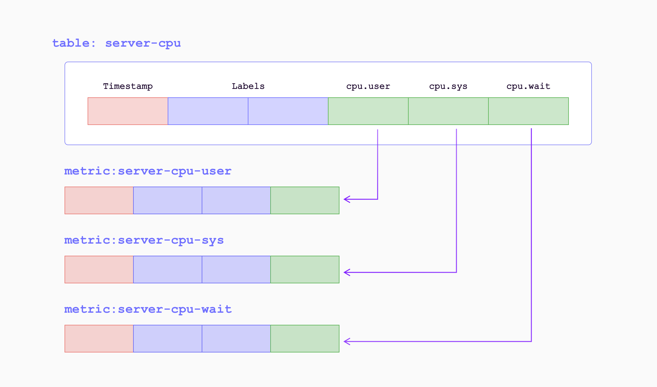
When the metrics are written into GreptimeDB by remote write endpoint, they will be transformed as
follows:
| Sample Metrics | In GreptimeDB | GreptimeDB Data Types |
| -------------- | ------------------------- | --------------------- |
| Name | Table (Auto-created) Name | String |
| Value | Column (Field) | Double |
| Timestamp | Column (Time Index) | Timestamp |
| Label | Column (Tag) | String |
For example, the following Prometheus metric:
```txt
prometheus_remote_storage_samples_total{instance="localhost:9090", job="prometheus",
remote_name="648f0c", url="http://localhost:4000/v1/prometheus/write"} 500
```
will be transformed as a row in the table `prometheus_remote_storage_samples_total`:
| Column | Value | Column Data Type |
| :----------------- | :------------------------------------------ | :----------------- |
| instance | localhost:9090 | String |
| job | prometheus | String |
| remote_name | 648f0c | String |
| url | `http://localhost:4000/v1/prometheus/write` | String |
| greptime_value | 500 | Double |
| greptime_timestamp | The sample's unix timestamp | Timestamp |
## Improve efficiency by using metric engine
The Prometheus remote writing always creates a large number of small tables.
These tables are classified as logical tables in GreptimeDB.
However, having a large number of small tables can be inefficient for both data storage and query performance.
To address this, GreptimeDB introduces the [metric engine](/contributor-guide/datanode/metric-engine.md) feature,
which stores the data represented by the logical tables in a single physical table.
This approach reduces storage overhead and improves columnar compression efficiency.
The metric engine is enabled by default in GreptimeDB,
and you don't need to specify any additional configuration.
By default, the physical table used is `greptime_physical_table`.
If you want to use a specific physical table, you can specify the `physical_table` parameter in the remote write URL.
If the specified physical table doesn't exist, it will be automatically created.
```yaml
remote_write:
- url: http://localhost:4000/v1/prometheus/write?db=public&physical_table=greptime_physical_table
```
Data is stored in the physical table,
while queries are performed on logical tables to provide an intuitive view from a metric perspective.
For instance, when successfully writing data, you can use the following command to display the logical tables:
```sql
show tables;
```
```sql
+---------------------------------------------------------------+
| Tables |
+---------------------------------------------------------------+
| prometheus_remote_storage_enqueue_retries_total |
| prometheus_remote_storage_exemplars_pending |
| prometheus_remote_storage_read_request_duration_seconds_count |
| prometheus_rule_group_duration_seconds |
| ...... |
+---------------------------------------------------------------+
```
The physical table itself can also be queried.
It contains columns from all the logical tables,
making it convenient for multi-join analysis and computation.
To view the schema of the physical table, use the `DESC TABLE` command:
```sql
DESC TABLE greptime_physical_table;
```
The physical table includes all the columns from the logical tables:
```sql
+--------------------+----------------------+------+------+---------+---------------+
| Column | Type | Key | Null | Default | Semantic Type |
+--------------------+----------------------+------+------+---------+---------------+
| greptime_timestamp | TimestampMillisecond | PRI | NO | | TIMESTAMP |
| greptime_value | Float64 | | YES | | FIELD |
| __table_id | UInt32 | PRI | NO | | TAG |
| __tsid | UInt64 | PRI | NO | | TAG |
| device | String | PRI | YES | | TAG |
| instance | String | PRI | YES | | TAG |
| job | String | PRI | YES | | TAG |
| error | String | PRI | YES | | TAG |
...
```
You can use the `SELECT` statement to filter data from the physical table as needed.
For example, you can filter data based on the `device` condition from logical table A and the `job` condition from logical table B:
```sql
SELECT *
FROM greptime_physical_table
WHERE greptime_timestamp > "2024-08-07 03:27:26.964000"
AND device = "device1"
AND job = "job1";
```
### GreptimeDB cluster with metric engine
If you are using GreptimeDB cluster for Prometheus remote write, you may notice
that only 1 datanode taking all the workload and other datanodes receives no
traffic. This is because with default settings, there is only 1 metric engine
physical table, and only 1 partition(region) in that table. The datanode that
serves the partition will take all the data ingestion.
Why we are not creating more partitions by default? [GreptimeDB's table
partition](/user-guide/deployments-administration/manage-data/table-sharding.md)
is based pre-configured partition columns. However, in Prometheus ecosystem,
there is no common column (label, as in Prometheus) that is suitable for good
partition rules.
To fix this, we recommend you to define your own partition rule based on your
data model. For example, it can be `namespace` if your are monitoring a
kubernetes cluster. The partition columns should have enough cardinality to
divide data. Also we recommend you to create 2x-3x partitions on initial
datanode count, so when you scaling more datanodes in your cluster, just migrate
those partitions to new ones.
An example DDL of partitioned physical table based on `namespace` label:
```sql
CREATE TABLE greptime_physical_table (
greptime_timestamp TIMESTAMP(3) NOT NULL,
greptime_value DOUBLE NULL,
namespace STRING PRIMARY KEY,
TIME INDEX (greptime_timestamp),
)
PARTITION ON COLUMNS (namespace) (
namespace <'g',
namespace >= 'g' AND namespace < 'n',
namespace >= 'n' AND namespace < 't',
namespace >= 't'
)
ENGINE = metric
with (
"physical_metric_table" = "",
);
```
Note that you won't have need add all possible *PRIMARY KEY* (label) here,
metric engine will add them automatically. Only labels you use for partitioning
are required to be defined ahead of time.
## Special labels for ingestion options
:::warning Experimental Feature
This experimental feature may contain unexpected behavior, have its functionality change in the future.
:::
Normally, the complete dataset of a remote write request is ingested into the database under the same option, for example, a default physical table with metric engine enabled.
All the logical tables (i.e, the metrics) is backed with the same physical table, even when the number of metrics grows.
It's probably fine for data ingestion. However, this set-up might slow down the query speed if you just want to query for a small group of metrics, but the database have to scan the complete dataset because they are all in the same physical table.
If you can foresee a large data volume and incremental queries upon a small group of metrics each time, then it might be useful to split the storage during the ingestion to reduce the query overhead later. This fine-grade level of control can be achieved using ingest options for each metric within a remote request.
Starting from `v0.15`, GreptimeDB is adding support for special labels.
There labels (along with there values) will turn into ingest options during the parsing phase, allowing individual metric within a request to be more precisely controlled.
The labels are not mutually exclusive, so they can be combined together to produce more versatile controlling.
Here is a representative diagram of special labels for a metric. Note this is not the actual data model of a metric.
| `__name__` | `x_greptime_database` | `x_greptime_physical_table` | `pod_name_label` | `__normal_label_with_underscore_prefix__` | `timestamp` | `value` |
|--------------------|-------------------------|-------------------------------|-----------------------|---------------------------------------------|---------------------------|-----------|
| `some_metric_name` | `public` | `p_1` | `random_k8s_pod_name` | `true` | `2025-06-17 16:31:52.000` | `12.1` |
The special labels you see above are just normal valid labels in Prometheus.
GreptimeDB recognizes some of the label names and turns them into ingest options.
It's much like the custom HTTP headers, where you just set a valid HTTP header and its value to indicate following operations, only the header pair means nothing outside your program.
Here is a list of supported label names:
- `x_greptime_database`
- `x_greptime_physical_table`
### Setting labels
How to set labels to the metrics is very dependent on the tools (or code) that collects the metrics and send them over to the database.
If you're using Prometheus to scrape metrics from the source and send them to GreptimeDB using remote write, you can add `external_labels` in the global config.
Refer to the [docs](https://prometheus.io/docs/prometheus/latest/configuration/configuration/#configuration-file) here.
It's the same for other collecting tools. You may have to find the relevant configuration for your tool of choice.
### `x_greptime_database`
This option decides which database the metric goes into. Note, the database should be created in advance(for instance, using `create database xxx` SQL).
Metrics from the same tech stack can have same metric names.
For example, if you have two Kubernetes clusters with very different content, and you deploy a single collector on both clusters, they will generate metrics with same names but with different labels or values.
If the metrics are collected and ingested into the same database, then on a Grafana dashboard you will have to manually set every label selection on every diagram to view the two clusters' metrics separately. This can be very tedious and painful.
In this case, you might want to store the metrics on different databases during ingestion and use two dashboards to view the metrics separately.
### `x_greptime_physical_table`
If the metric is storing using the metric engine, then there is a physical table behind each metric's logical table.
By default, all metrics using the same physical table.
With the number of the metrics growing, this physical table becomes a super wide table.
If the metric frequency is different, then the table will be sparse.
Finding a certain metric or a certain label in the complete metrics dataset would be very time-consuming since the database have to scan all the 'irrelevant' data.
In this case, you might want to split the metrics into different physical tables to ease the pressure on a single physical table.
It can also be helpful to group metrics by their frequency.
Note, each metric's logical table is bound to a physical table upon creation.
So setting different physical table for the same metric within the same database won't work.
## Using pipeline in remote write
:::warning Experimental Feature
This experimental feature may contain unexpected behavior, have its functionality change in the future.
:::
Starting from `v0.15`, GreptimeDB supports using pipeline to process Prometheus remote write requests.
You can simply set the HTTP header `x-greptime-pipeline-name` to the target pipeline name to enable pipeline processing.
Here is a very simple pipeline configuration, using `vrl` processor to add a `source` label to each metric:
```YAML
version: 2
processors:
- vrl:
source: |
.source = "local_laptop"
.
transform:
- field: greptime_timestamp
type: time, ms
index: timestamp
```
The result looks something like this
```
mysql> select * from `go_memstats_mcache_inuse_bytes`;
+----------------------------+----------------+--------------------+---------------+--------------+
| greptime_timestamp | greptime_value | instance | job | source |
+----------------------------+----------------+--------------------+---------------+--------------+
| 2025-07-11 07:42:03.064000 | 1200 | node_exporter:9100 | node-exporter | local_laptop |
| 2025-07-11 07:42:18.069000 | 1200 | node_exporter:9100 | node-exporter | local_laptop |
+----------------------------+----------------+--------------------+---------------+--------------+
2 rows in set (0.01 sec)
```
You can refer to the [pipeline's documentation](/user-guide/logs/use-custom-pipelines.md) for more details.
## Performance tuning
By default, the metric engine will automatically create a physical table named `greptime_physical_table` if it does not already exist. For performance optimization, you may choose to create a physical table with customized configurations.
### Enable skipping index
By default, the metric engine won't create indexes for columns. You can enable it by setting the `index.type` to `skipping`.
Create a physical table with a skipping index; all automatically added columns will have this index applied.
```sql
CREATE TABLE greptime_physical_table (
greptime_timestamp TIMESTAMP(3) NOT NULL,
greptime_value DOUBLE NULL,
TIME INDEX (greptime_timestamp),
)
engine = metric
with (
"physical_metric_table" = "",
"index.type" = "skipping"
);
```
For more configurations, please refer to the [create table](/reference/sql/create.md#create-table) section.
## VictoriaMetrics remote write
VictoriaMetrics slightly modified Prometheus remote write protocol for better
compression. The protocol is automatically enabled when you are using `vmagent`
to send data to a compatible backend.
GreptimeDB has this variant supported, too. Just configure GreptimeDB's remote
write url for `vmagent`. For example, if you have GreptimeDB installed locally:
```shell
vmagent -remoteWrite.url=http://localhost:4000/v1/prometheus/write
```
---
## Vector
:::tip NOTE
This document is based on Vector v0.49.0. All example configurations below are based on this version. Please adjust the host and port configurations for each sink according to your actual GreptimeDB instance. All port values below are defaults.
:::
Vector is a high-performance observability data pipeline. It natively supports GreptimeDB as a metrics data receiver. Through Vector, you can receive metrics data from various sources including Prometheus, OpenTelemetry, StatsD, etc. GreptimeDB can serve as a sink component for Vector to receive metrics data.
## Writing Metrics Data
GreptimeDB supports multiple ways to write metrics data:
- Using [`greptimedb_metrics` sink](https://vector.dev/docs/reference/configuration/sinks/greptimedb_metrics/)
- Using InfluxDB line protocol format
- Using Prometheus Remote Write protocol
### Using `greptimedb_metrics` sink
#### Example
Below is an example configuration using `greptimedb_metrics` sink to write host metrics:
```toml
# sample.toml
[sources.in]
type = "host_metrics"
[sinks.my_sink_id]
inputs = ["in"]
type = "greptimedb_metrics"
endpoint = ":4001"
dbname = ""
username = ""
password = ""
new_naming = true
```
Vector uses gRPC to communicate with GreptimeDB, so the default port for Vector sink is `4001`. If you changed the default gRPC port when starting GreptimeDB with [custom configuration](/user-guide/deployments-administration/configuration.md#configuration-file), please use your own port.
For more requirements, please visit [Vector GreptimeDB Configuration](https://vector.dev/docs/reference/configuration/sinks/greptimedb_metrics/) to view more configuration options.
### Data Model
The following rules are used when storing Vector metrics into GreptimeDB:
- Use `_` as the table name in GreptimeDB, for example, `host_cpu_seconds_total`;
- Use the timestamp of the metric as the time index of GreptimeDB, the column name is `ts`;
- Use the tags of the metric as GreptimeDB tags;
- For Vector metrics which have multiple subtypes:
- For Counter and Gauge metrics, the values are stored in the `val` column;
- For Set metrics, the number of data points are stored in the `val` column;
- For Distribution metrics, the values of each percentile are stored in the `pxx` column, where xx is the percentile, and the `min/max/avg/sum/count` columns are also stored;
- For AggregatedHistogram metrics, the values of each bucket are stored in the `bxx` column, where xx is the upper limit of the bucket, and the `sum/count` columns are also stored;
- For AggregatedSummary metrics, the values of each percentile are stored in the `pxx` column, where xx is the percentile, and the `sum/count` columns are also stored;
- For Sketch metrics, the values of each percentile are stored in the `pxx` column, where xx is the percentile, and the `min/max/avg/sum` columns are also stored;
### Using InfluxDB Line Protocol Format
You can use the `influx` sink to write metrics data. We recommend using v2 version of InfluxDB line protocol format.
Below is an example configuration using `influx` sink to write host metrics:
```toml
# sample.toml
[sources.my_source_id]
type = "internal_metrics"
[sinks.my_sink_id]
type = "influxdb_metrics"
inputs = [ "my_source_id" ]
bucket = "public"
endpoint = "http://:4000/v1/influxdb"
org = ""
token = ""
```
The above configuration uses v2 version of InfluxDB line protocol. Vector determines the InfluxDB protocol version based on fields in the TOML configuration, so please ensure the configuration contains `bucket`, `org`, and `token` fields. Specific field explanations:
- `type`: Value for InfluxDB line protocol is `influxdb_metrics`.
- `bucket`: Database name in GreptimeDB.
- `org`: Organization name in GreptimeDB (needs to be empty).
- `token`: Token for authentication (needs to be empty). Since Influx line protocol token has special format and must start with `Token `, this differs from GreptimeDB's authentication method and is currently not compatible. If using GreptimeDB instance with authentication, please use `greptimedb_metrics`.
For more details, please refer to [InfluxDB Line Protocol documentation](../for-iot/influxdb-line-protocol.md) to learn how to write data to GreptimeDB using InfluxDB Line Protocol.
### Using Prometheus Remote Write Protocol
Below is an example configuration using Prometheus Remote Write protocol to write host metrics:
```toml
# sample.toml
[sources.my_source_id]
type = "internal_metrics"
[sinks.prometheus_remote_write]
type = "prometheus_remote_write"
inputs = [ "my_source_id" ]
endpoint = "http://:4000/v1/prometheus/write?db="
compression = "snappy"
auth = { strategy = "basic", username = "", password = "" }
```
## Writing Logs Data
GreptimeDB supports multiple ways to write logs data:
- Using [`greptimedb_logs` sink](https://vector.dev/docs/reference/configuration/sinks/greptimedb_logs/) to write logs data to GreptimeDB.
- Using Loki protocol to write logs data to GreptimeDB.
We strongly recommend all users to use `greptimedb_logs` sink to write logs data, as it is optimized for GreptimeDB and better supports GreptimeDB features. We also recommend enabling compression for various protocols to improve data transmission efficiency.
### Using `greptimedb_logs` sink (recommended)
```toml
# sample.toml
[sources.my_source_id]
type = "demo_logs"
count = 10
format = "apache_common"
interval = 1
[sinks.my_sink_id]
type = "greptimedb_logs"
inputs = [ "my_source_id" ]
compression = "gzip"
dbname = "public"
endpoint = "http://:4000"
extra_headers = { "skip_error" = "true" }
pipeline_name = "greptime_identity"
table = ""
username = ""
password = ""
[sinks.my_sink_id.extra_params]
source = "vector"
x-greptime-pipeline-params = "max_nested_levels=10"
```
This example demonstrates how to use `greptimedb_logs` sink to write generated demo logs data to GreptimeDB. For more information, please refer to [Vector greptimedb_logs sink](https://vector.dev/docs/reference/configuration/sinks/greptimedb_logs/) documentation.
### Using Loki Protocol
#### Example
```toml
[sources.generate_syslog]
type = "demo_logs"
format = "syslog"
count = 100
interval = 1
[transforms.remap_syslog]
inputs = ["generate_syslog"]
type = "remap"
source = """
.labels = {
"host": .host,
"service": .service,
}
.structured_metadata = {
"source_type": .source_type
}
"""
[sinks.my_sink_id]
type = "loki"
inputs = ["remap_syslog"]
compression = "snappy"
endpoint = "http://:4000"
out_of_order_action = "accept"
path = "/v1/loki/api/v1/push"
encoding = { codec = "raw_message" }
labels = { "*" = "{{labels}}" }
structured_metadata = { "*" = "{{structured_metadata}}" }
auth = {strategy = "basic", user = "", password = ""}
```
The above configuration writes logs data to GreptimeDB using Loki protocol. Specific configuration item explanations:
- `compression`: Sets compression algorithm for data transmission, using `snappy` here.
- `endpoint`: Specifies Loki's receiving address.
- `out_of_order_action`: Sets how to handle out-of-order logs, choosing `accept` here to accept out-of-order logs. GreptimeDB supports writing out-of-order logs.
- `path`: Specifies Loki's API path.
- `encoding`: Sets data encoding method, using `raw_message` here.
- `labels`: Specifies log labels, mapping `labels` content to `{{labels}}` here. That is the `labels` field in remap_syslog.
- `structured_metadata`: Specifies structured metadata, mapping `structured_metadata` content to `{{structured_metadata}}` here. That is the `structured_metadata` field in remap_syslog.
For meanings of `labels` and `structured_metadata`, please refer to [Loki documentation](https://grafana.com/docs/loki/latest/get-started/labels/bp-labels/).
For Loki protocol, `labels` will use Tag type in time series scenarios by default, please avoid using high-cardinality fields for these fields. `structured_metadata` will be stored as a complete JSON field.
Note that since Vector's configuration doesn't allow setting headers, you cannot specify pipeline. If you need to use pipeline functionality, please consider using `greptimedb_logs` sink.
---
## Ingest Data
GreptimeDB supports automatic schema generation and flexible data ingestion methods,
enabling you to easily write data tailored to your specific scenarios.
## Automatic Schema Generation
GreptimeDB supports schemaless writing, automatically creating tables and adding necessary columns as data is ingested.
This capability ensures that you do not need to manually define schemas beforehand, making it easier to manage and integrate diverse data sources seamlessly.
This feature is supported for all protocols and integrations, except [SQL](./for-iot/sql.md).
## Recommended Data Ingestion Methods
GreptimeDB supports various data ingestion methods for specific scenarios, ensuring optimal performance and integration flexibility.
- [For Observability Scenarios](./for-observability/overview.md): Suitable for real-time monitoring and alerting.
- [For IoT Scenarios](./for-iot/overview.md): Suitable for real-time data and complex IoT infrastructures.
## Next Steps
- [Query Data](/user-guide/query-data/overview.md): Learn how to explore your data by querying your GreptimeDB database.
- [Manage Data](/user-guide/manage-data/overview.md): Learn how to update and delete data, etc., to ensure data integrity and efficient data management.
---
## Grafana Alloy(Integrations)
GreptimeDB can be set up as a data sink for Grafana Alloy.
For more information, please refer to the [Ingest Data through Grafana Alloy](/user-guide/ingest-data/for-observability/alloy.md) guide.
---
## Coroot
Coroot is an open-source APM & Observability tool,
a DataDog and NewRelic alternative. Metrics, logs, traces, continuous profiling,
and SLO-based alerting, supercharged with predefined dashboards and inspections.
GreptimeDB can be configured as a Prometheus data sink for Coroot.
To integrate GreptimeDB with Coroot, navigate to `Settings` in the Coroot Dashboard,
select the `Prometheus` configuration, and enter the following information:
- Prometheus URL: `http{s}:///v1/prometheus`
- If you have [enabled authentication](/user-guide/deployments-administration/authentication/static.md) on GreptimeDB, check the HTTP basic auth option and enter GreptimeDB username and password. Otherwise, leave it unchecked.
- Remote Write URL: `http{s}:///v1/prometheus/write?db=`
## Example Configuration
If your GreptimeDB host is `localhost` with port `4000` for the HTTP service and authentication is enabled,
and you want to use the default database `public`,
use the following configuration:
- Prometheus URL: `http://localhost:4000/v1/prometheus`
- Enable the HTTP basic auth option and enter GreptimeDB username and password
- Remote Write URL: `http://localhost:4000/v1/prometheus/write?db=public`
The image below shows the Coroot configuration example:
Once the configuration is saved successfully,
you can begin using Coroot to monitor your instances.
The image below shows an example of a Coroot dashboard using GreptimeDB as a data source:
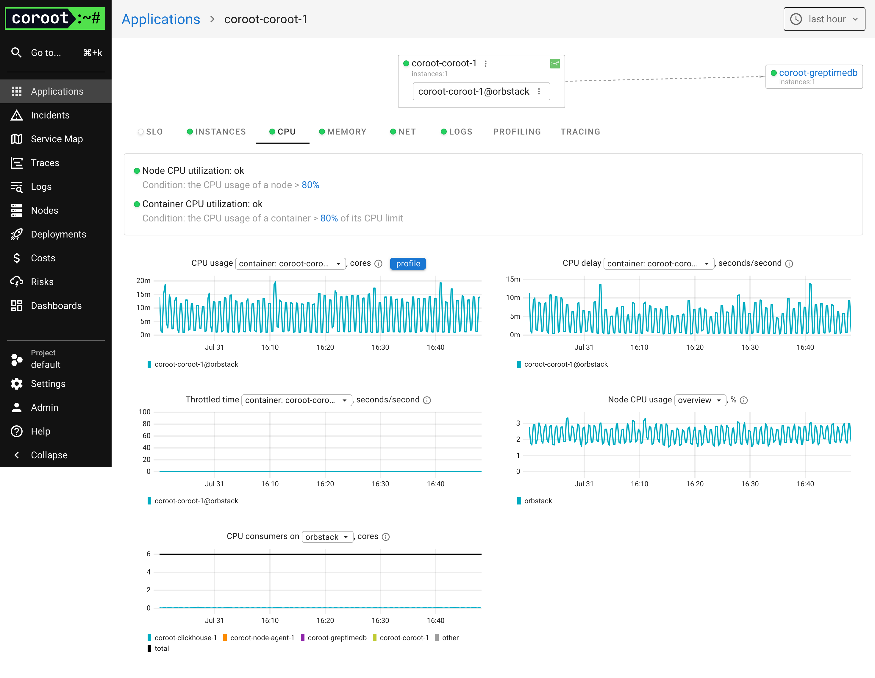
---
## DBeaver
[DBeaver](https://dbeaver.io/) is a free, open-source, and cross-platform database tool that supports all popular databases. It is a popular choice among developers and database administrators for its ease of use and extensive feature set.
You can use DBeaver to connect to GreptimeDB via MySQL database drivers.
Click the "New Database Connection" button in the DBeaver toolbar to create a new connection to GreptimeDB.
Select MySQL and click "Next" to configure the connection settings.
Install the MySQL driver if you haven't already.
Input the following connection details:
- Connect by Host
- Host: `localhost` if GreptimeDB is running on your local machine
- Port: `4002` if you use the default GreptimeDB configuration
- Database: `public`, you can use any other database name you have created
- Enter the username and password if authentication is enabled on GreptimeDB; otherwise, leave them blank.
Click "Test Connection" to verify the connection settings and click "Finish" to save the connection.
For more information on interacting with GreptimeDB using MySQL, refer to the [MySQL protocol documentation](/user-guide/protocols/mysql.md).
---
## EMQX(Integrations)
GreptimeDB can be used as a data system for EMQX.
For more information, please refer to the [Ingest Data through EMQX](/user-guide/ingest-data/for-iot/emqx.md) guide.
---
## Fluent Bit(Integrations)
You can set GreptimeDB as a Output for Fluent Bit.
For more information, please refer to the [Writing Data with Fluent Bit](../ingest-data/for-observability/fluent-bit.md) guide.
---
## Grafana
GreptimeDB can be configured as a [Grafana data source](https://grafana.com/docs/grafana/latest/datasources/add-a-data-source/).
You have the option to connect GreptimeDB with Grafana using one of three data sources: [GreptimeDB](#greptimedb-data-source-plugin), [Prometheus](#prometheus-data-source), or [MySQL](#mysql-data-source).
## GreptimeDB data source plugin
The [GreptimeDB data source plugin](https://github.com/GreptimeTeam/greptimedb-grafana-datasource) is based on the ClickHouse data source and adds GreptimeDB-specific features.
The plugin adapts perfectly to the GreptimeDB data model,
thus providing a better user experience.
In addition, it also solves some compatibility issues compared to using the Prometheus data source directly.
### Installation
The GreptimeDB Data source plugin can currently only be installed on a local Grafana instance.
Make sure Grafana is installed and running before installing the plugin.
You can choose one of the following installation methods:
- Download the installation package and unzip it to the relevant directory: Grab the latest release from [release
page](https://github.com/GreptimeTeam/greptimedb-grafana-datasource/releases/latest/),
Unzip the file to your [grafana plugin
directory](https://grafana.com/docs/grafana/latest/setup-grafana/configure-grafana/#plugins).
- Use grafana cli to download and install:
```shell
grafana cli --pluginUrl https://github.com/GreptimeTeam/greptimedb-grafana-datasource/releases/latest/download/info8fcc-greptimedb-datasource.zip plugins install info8fcc
```
- Use our [prebuilt Grafana docker
image](https://hub.docker.com/r/greptime/grafana-greptimedb), which ships the
plugin by default: `docker run -p 3000:3000
greptime/grafana-greptimedb:latest`
Note that you may need to restart your grafana server after installing the plugin.
### Connection settings
Click the Add data source button and select GreptimeDB as the type.
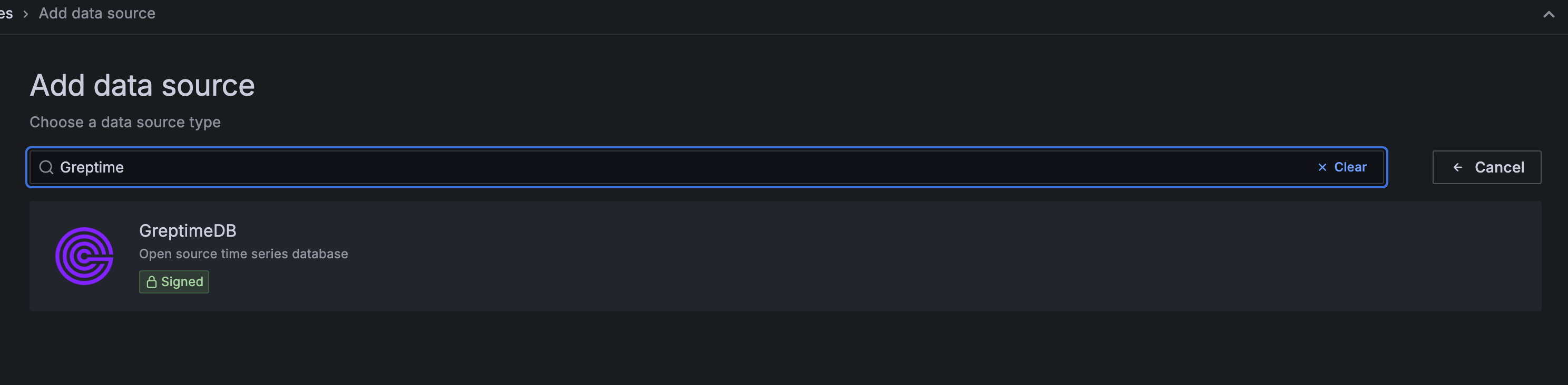
Fill in the following URL in the GreptimeDB server URL:
```txt
http://:4000
```
In the Auth section, click basic auth, and fill in the username and password for GreptimeDB in the Basic Auth Details section (not set by default, no need to fill in).
- User: ``
- Password: ``
Then click the Save & Test button to test the connection.
### General Query Settings
Before selecting any query type, you first need to configure the **Database** and **Table** to query from.
| Setting | Description |
| :-------- | :---------------------------------------- |
| **Database** | Select the database you want to query. |
| **Table** | Select the table you want to query from. |

---
### Table Query
Choose the `Table` query type when your query results **do not include a time column**. This is suitable for displaying tabular data.
| Setting | Description |
| :-------- | :---------------------------------------------- |
| **Columns** | Select the columns you want to retrieve. Multiple selections are allowed. |
| **Filters** | Set conditions to filter your data. |
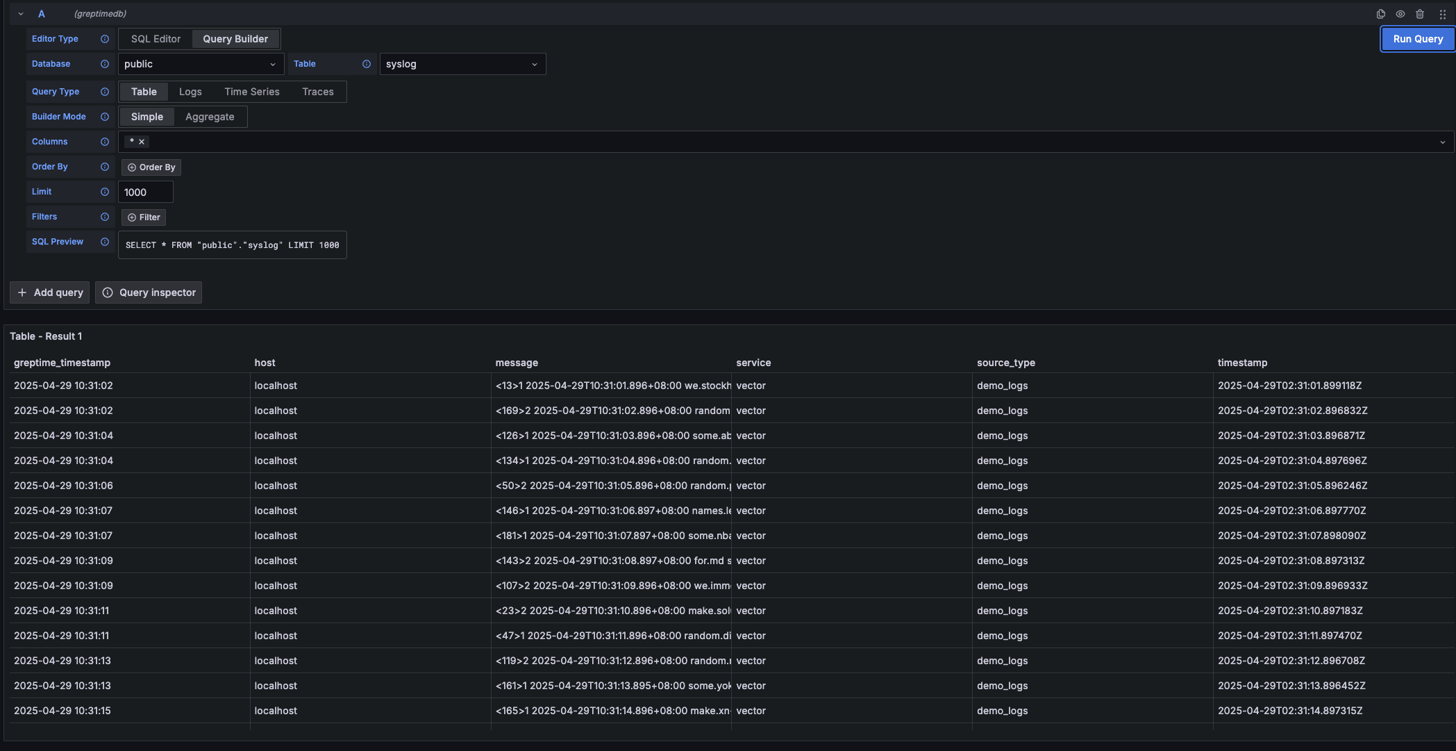
---
### Metrics Query
Select the `Time Series` query type when your query results **include both a time column and a numerical value column**. This is ideal for visualizing metrics over time.
| Main Setting | Description |
| :----------- | :-------------------- |
| **Time** | Select the time column. |
| **Columns** | Select the numerical value column(s). |
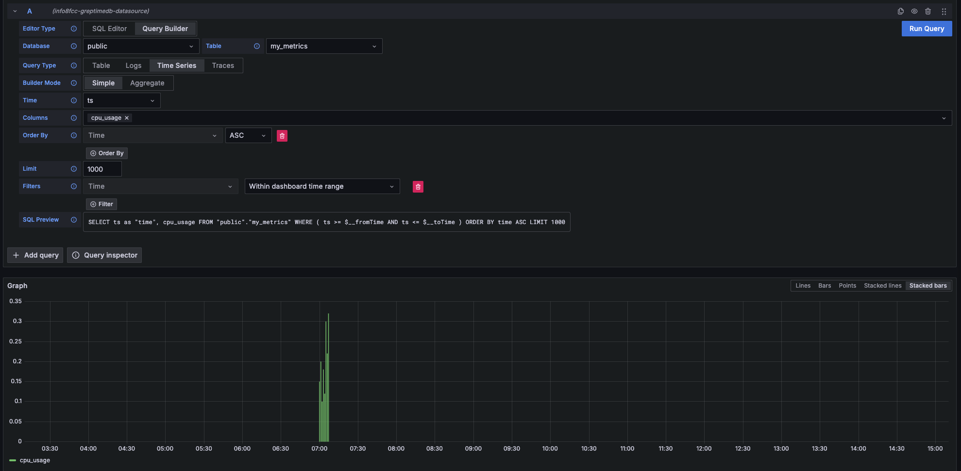
---
### Logs Query
Choose the `Logs` query type when you want to query log data. You'll need to specify a **Time** column and a **Message** column.
| Main Setting | Description |
| :----------- | :---------------------------- |
| **Time** | Select the timestamp column for your logs. |
| **Message** | Select the column containing the log content. |
| **Log Level**| (Optional) Select the column representing the log level. |
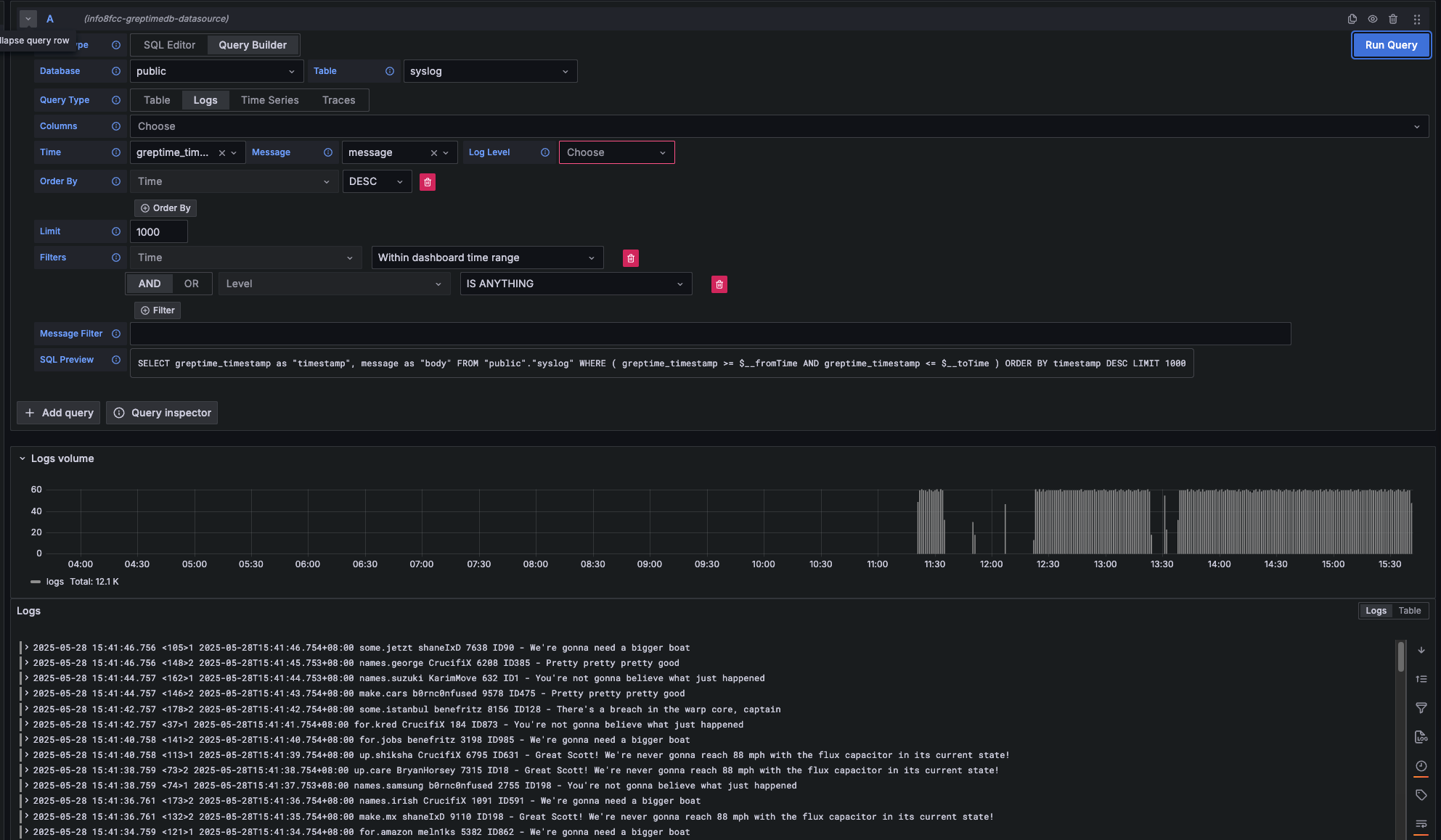
#### logs Context Query
Logs Context Query
Performs an approximate time range query based on the value of context columns in a log row.
* First, set the context column in Connection Page.
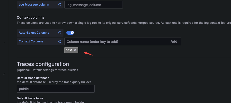
* Then, when making a query, include the context column in the query.
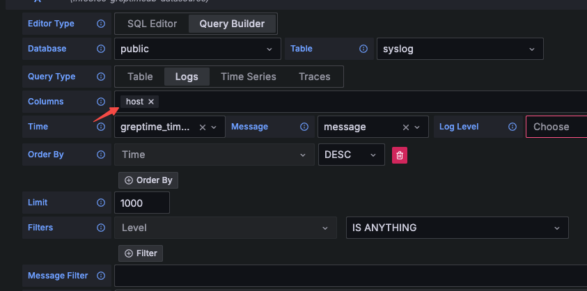
---
### Traces Query
Select the `Traces` query type when you want to query distributed tracing data.
| Main Setting | Description |
| :-------------------- | :------------------------------------------------------------------------------------------------------ |
| **Trace Model** | Select `Trace Search` to query a list of traces. |
| **Trace Id Column** | Default value: `trace_id` |
| **Span Id Column** | Default value: `span_id` |
| **Parent Span ID Column** | Default value: `parent_span_id` |
| **Service Name Column** | Default value: `service_name` |
| **Operation Name Column** | Default value: `span_name` |
| **Start Time Column** | Default value: `timestamp` |
| **Duration Time Column** | Default value: `duration_nano` |
| **Duration Unit** | Default value: `nano_seconds` |
| **Tags Column** | Multiple selections allowed. Corresponds to columns starting with `span_attributes` (e.g., `span_attributes.http.method`). |
| **Service Tags Column** | Multiple selections allowed. Corresponds to columns starting with `resource_attributes` (e.g., `resource_attributes.host.name`). |
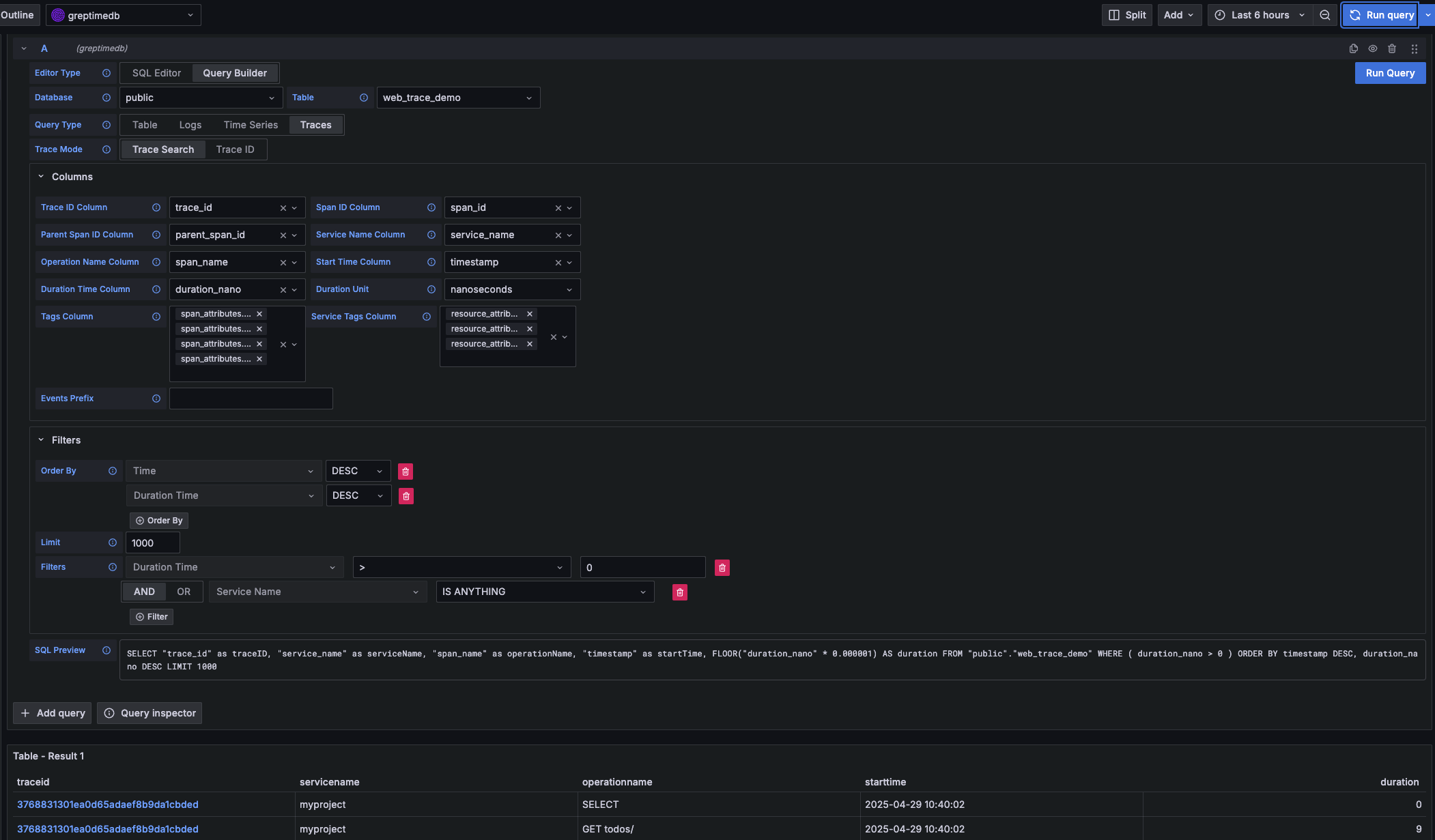
## Prometheus data source
Click the "Add data source" button and select Prometheus as the type.
Fill in Prometheus server URL in HTTP:
```txt
http://:4000/v1/prometheus
```
Click basic auth in the Auth section and fill in your GreptimeDB username and password in Basic Auth Details:
- User: ``
- Password: ``
Click Custom HTTP Headers and add one header:
- Header: `x-greptime-db-name`
- Value: ``
Then click "Save & Test" button to test the connection.
For how to query data with PromQL, please refer to the [Prometheus Query Language](/user-guide/query-data/promql.md) document.
## MySQL data source
Click the "Add data source" button and select MySQL as the type. Fill in the following information in MySQL Connection:
- Host: `:4002`
- Database: ``
- User: ``
- Password: ``
- Session timezone: `UTC`
Then click "Save & Test" button to test the connection.
Note that you need to use raw SQL editor for panel creation. SQL Builder is not
supported due to timestamp data type difference between GreptimeDB and vanilla
MySQL.
For how to query data with SQL, please refer to the [Query Data with SQL](/user-guide/query-data/sql.md) document.
---
## Kafka(Integrations)
Vector can be used as a tool to transport data from Kafka to GreptimeDB.
For more information, please refer to the [Ingest Data via Kafka](/user-guide/ingest-data/for-observability/kafka.md) guide.
---
## Model Context Protocol (MCP)
:::warning Experimental Feature
The GreptimeDB MCP Server is currently in experimental stage and under active development. APIs and features may change without notice. Please use with caution in production environments.
:::
The [GreptimeDB MCP Server](https://github.com/GreptimeTeam/greptimedb-mcp-server) provides a Model Context Protocol implementation that enables AI assistants like Claude to securely explore and analyze your GreptimeDB databases.
Watch our [demo video on YouTube](https://www.youtube.com/watch?v=EBTc46yamFI) to see the MCP Server in action and get a better understanding of its capabilities.
## What is MCP?
Model Context Protocol (MCP) is a standard protocol that allows AI assistants to interact with external data sources and tools. With the GreptimeDB MCP Server, you can enable AI assistants to:
- List and explore database tables
- Read table data and schemas
- Execute SQL queries
- Analyze time-series data through natural language
## Installation
Install the GreptimeDB MCP Server using pip:
```bash
pip install greptimedb-mcp-server
```
## Configuration
The MCP server can be configured through environment variables or command-line arguments. Key configuration options include:
- Database connection settings (host, port, username, password)
- Database name
- Timezone settings
### Example: Claude Desktop Integration
To integrate with Claude Desktop, add the following configuration to your `claude_desktop_config.json`:
```json
{
"mcpServers": {
"greptimedb": {
"command": "python",
"args": ["-m", "greptimedb_mcp_server"],
"env": {
"GREPTIMEDB_HOST": "localhost",
"GREPTIMEDB_PORT": "4002",
"GREPTIMEDB_USERNAME": "your_username",
"GREPTIMEDB_PASSWORD": "your_password",
"GREPTIMEDB_DATABASE": "your_database"
}
}
}
}
```
## Learn More
For detailed configuration options, advanced usage, and troubleshooting, refer to the [GreptimeDB MCP Server documentation](https://github.com/GreptimeTeam/greptimedb-mcp-server).
:::note
The GreptimeDB MCP Server is an experimental project still under development. Exercise caution when using it with sensitive data.
:::
---
## Metabase
[Metabase](https://github.com/metabase/metabase) is an open source BI tool that
written in Clojure. You can configure GreptimeDB as a metabase data source from
a community driver plugin.
## Installation
Download the driver plugin file `greptimedb.metabase-driver.jar` from its
[release
page](https://github.com/greptimeteam/greptimedb-metabase-driver/releases/latest/). Copy
the jar file to `plugins/` of metabase's working directory. It will be
discovered by Metabase automatically.
## Add GreptimeDB as database
To add GreptimeDB database, select *Settings* / *Admin Settings* / *Databases*,
click *Add Database* button and select GreptimeDB from *Database type*.
You will be asked to provide host, port, database name and authentication
information.
- Use Greptime's Postgres protocol port `4003` as port. If you changed the
defaults, use you own settings.
- Username and password are optional if you didn't enable
[authentication](/user-guide/deployments-administration/authentication/overview.md).
- Use `public` as default *Database name*. When using GreptimeCloud instance,
use the database name from your instance.
---
## MindsDB
[MindsDB](https://mindsdb.com/) is an open-source machine learning platform that
enables developers to easily incorporate advanced machine learning capabilities
with existing databases.
Your GreptimeDB instance work out of box as using GreptimeDB extension with
MindsDB. You can configure GreptimeDB as a data source in MindsDB using MySQL protocol:
```sql
CREATE DATABASE greptime_datasource
WITH ENGINE = 'greptimedb',
PARAMETERS = {
"host": "",
"port": 4002,
"database": "",
"user": "",
"password": "",
"ssl": True
};
```
- `` is the hostname or IP address of your GreptimeDB instance.
- `` is the name of the database you want to connect to.
- `` and `` are your [GreptimeDB credentials](/user-guide/deployments-administration/authentication/static.md).
MindsDB is a great gateway for many machine learning features, including
time-series forecasting, for your time series data stored in our instance. See
[MindsDB docs](https://docs.mindsdb.com/what-is-mindsdb) for more information.
---
## Integrations
GreptimeDB can be seamlessly integrated with popular tools for data ingestion, querying, and visualization.
The subsequent sections offer comprehensive guidance on integrating GreptimeDB with the following tools:
---
## Prometheus(Integrations)
## Remote Write
GreptimeDB can be used as a remote storage backend for Prometheus.
For detailed information,
please refer to the [Ingest Data with Prometheus Remote Write](/user-guide/ingest-data/for-observability/prometheus.md) document.
## Prometheus Query Language (PromQL)
GreptimeDB supports the Prometheus Query Language (PromQL) for querying metrics.
For more information,
please refer to the [Query Data with Prometheus Query Language](/user-guide/query-data/promql.md) document.
---
## Streamlit
[Streamlit](https://streamlit.io/) is a faster way to build and share data apps.
It's possible to build streamlit based data apps based on GreptimeDB.
To use GreptimeDB data in your application, you will need to create a SQL
connection. Thanks to GreptimeDB's [MySQL protocol compatibility](/user-guide/protocols/mysql.md),
you can treat GreptimeDB as MySQL when connecting to it.
Here is an example code snippet to connect to GreptimeDB from Streamlit:
```python
st.title('GreptimeDB Streamlit Demo')
conn = st.connection("greptimedb", type="sql", url="mysql://:@:4002/")
df = conn.query("SELECT * FROM ...")
```
- The `` is the hostname or IP address of your GreptimeDB instance.
- The `` is the name of the database you want to connect to.
- The `` and `` are your [GreptimeDB credentials](/user-guide/deployments-administration/authentication/static.md).
Once you have created the connection, you can run SQL query against your
GreptimeDB instance. The resultset is automatically converted to Pandas
dataframe just like normal data source in streamlit.
---
## Superset
[Apache Superset](https://superset.apache.org) is an open source BI tool that
written in Python. To configure GreptimeDB as a database in Superset, you can
follow this guide.
## Installation
### Running Superset with Docker Compose
[Docker compose](https://superset.apache.org/docs/installation/docker-compose)
is the recommended way to run Superset. To add GreptimeDB extension, create a
`requirements-local.txt` file in `docker/` of Superset codebase.
Add GreptimeDB dependency in `requirements-local.txt`:
```txt
greptimedb-sqlalchemy
```
Start Superset services:
```bash
docker compose -f docker-compose-non-dev.yml up
```
### Running Superset Locally
If you are [running Superset from
pypi](https://superset.apache.org/docs/installation/pypi), install our extension
to the same environment.
```bash
pip install greptimedb-sqlalchemy
```
## Add GreptimeDB as database
To add GreptimeDB database, select *Settings* / *Database Connections*.
Add database and select *GreptimeDB* from list of supported databases.
Follow the SQLAlchemy URI pattern to provide your connection information:
```
greptimedb://:@:/
```
- Ignore `:@` if you don't have
[authentication](/user-guide/deployments-administration/authentication/overview.md) enabled.
- Use `4003` for default port (this extension uses Postgres protocol).
- Use `public` as default `database`. When using GreptimeCloud instance, use the
database name from your instance.
---
## Telegraf
For instructions on how to write data to GreptimeDB using Telegraf, please refer to the [Telegraf section](/user-guide/ingest-data/for-iot/influxdb-line-protocol.md#telegraf) in the InfluxDB Line Protocol documentation.
---
## Vector(Integrations)
Please refer to the [Ingest Data with Vector](/user-guide/ingest-data/for-observability/vector.md) document for instructions on how to sink data to GreptimeDB using Vector.
---
## Full-Text Search
This document provides a guide on how to use GreptimeDB's query language for effective searching and analysis of log data.
GreptimeDB allows for flexible querying of data using SQL statements. This section introduces specific search functions and query statements designed to enhance your log querying capabilities.
## Pattern Matching Using the `matches_term` Function
In SQL statements, you can use the `matches_term` function to perform exact term/phrase matching, which is especially useful for log analysis. The `matches_term` function supports pattern matching on `String` type columns. You can also use the `@@` operator as a shorthand for `matches_term`. Here's an example of how it can be used:
```sql
-- Using matches_term function
SELECT * FROM logs WHERE matches_term(message, 'error') OR matches_term(message, 'fail');
-- Using @@ operator (shorthand for matches_term)
SELECT * FROM logs WHERE message @@ 'error' OR message @@ 'fail';
```
The `matches_term` function is designed for exact term/phrase matching and uses the following syntax:
- `text`: The text column to search, which should contain textual data of type `String`.
- `term`: The search term or phrase to match exactly, following these rules:
- Case-sensitive matching
- Matches must have non-alphanumeric boundaries (start/end of text or any non-alphanumeric character)
- Supports whole-word matching and phrase matching
## Query Statements
### Simple Term Matching
The `matches_term` function performs exact word matching, which means it will only match complete words that are properly bounded by non-alphanumeric characters or the start/end of the text. This is particularly useful for finding specific error messages, status codes, version numbers, or paths in logs.
Error messages:
```sql
-- Using matches_term function
SELECT * FROM logs WHERE matches_term(message, 'error');
-- Using @@ operator
SELECT * FROM logs WHERE message @@ 'error';
```
Examples of matches and non-matches:
- ✅ "An error occurred!" - matches because "error" is a complete word
- ✅ "Critical error: system failure" - matches because "error" is bounded by space and colon
- ✅ "error-prone" - matches because "error" is bounded by hyphen
- ❌ "errors" - no match because "error" is part of a larger word
- ❌ "error123" - no match because "error" is followed by numbers
- ❌ "errorLogs" - no match because "error" is part of a camelCase word
File paths and commands:
```sql
-- Find specific command with path
SELECT * FROM logs WHERE matches_term(message, '/start');
```
Examples of matches and non-matches for '/start':
- ✅ "GET /app/start" - matches because "/start" is a complete term
- ✅ "Command: /start-process" - matches because "/start" is bounded by hyphen
- ✅ "Command: /start" - matches because "/start" is at the end of the message
- ❌ "start" - no match because it's missing the leading slash
- ❌ "start/stop" - no match because "/start" is not a complete term
### Multiple Term Searches
You can combine multiple `matches_term` conditions using the `OR` operator to search for logs containing any of several terms. This is useful when you want to find logs that might contain different variations of an error or different types of issues.
```sql
-- Using matches_term function
SELECT * FROM logs WHERE matches_term(message, 'critical') OR matches_term(message, 'error');
-- Using @@ operator
SELECT * FROM logs WHERE message @@ 'critical' OR message @@ 'error';
```
This query will find logs containing either "critical" or "error" as complete words. Each term is matched independently, and the results include logs that match either condition.
Examples of matches and non-matches:
- ✅ "critical error: system failure" - matches both terms
- ✅ "An error occurred!" - matches "error"
- ✅ "critical failure detected" - matches "critical"
- ❌ "errors" - no match because "error" is part of a larger word
- ❌ "critical_errors" - no match because terms are part of larger words
### Exclusion Searches
You can use the `NOT` operator with `matches_term` to exclude certain terms from your search results. This is useful when you want to find logs containing one term but not another.
```sql
-- Using matches_term function
SELECT * FROM logs WHERE matches_term(message, 'error') AND NOT matches_term(message, 'critical');
-- Using @@ operator
SELECT * FROM logs WHERE message @@ 'error' AND NOT message @@ 'critical';
```
This query will find logs containing the word "error" but not containing the word "critical". This is particularly useful for filtering out certain types of errors or focusing on specific error categories.
Examples of matches and non-matches:
- ✅ "An error occurred!" - matches because it contains "error" but not "critical"
- ❌ "critical error: system failure" - no match because it contains both terms
- ❌ "critical failure detected" - no match because it contains "critical"
### Required Term Searches
You can use the `AND` operator to require that multiple terms be present in the log message. This is useful for finding logs that contain specific combinations of terms.
```sql
-- Using matches_term function
SELECT * FROM logs WHERE matches_term(message, 'critical') AND matches_term(message, 'error');
-- Using @@ operator
SELECT * FROM logs WHERE message @@ 'critical' AND message @@ 'error';
```
This query will find logs containing both "critical" and "error" as complete words. Both conditions must be satisfied for a log to be included in the results.
Examples of matches and non-matches:
- ✅ "critical error: system failure" - matches because it contains both terms
- ❌ "An error occurred!" - no match because it only contains "error"
- ❌ "critical failure detected" - no match because it only contains "critical"
### Phrase Matching
The `matches_term` function can also match exact phrases, including those with spaces. This is useful for finding specific error messages or status updates that contain multiple words.
```sql
-- Using matches_term function
SELECT * FROM logs WHERE matches_term(message, 'system failure');
-- Using @@ operator
SELECT * FROM logs WHERE message @@ 'system failure';
```
This query will find logs containing the exact phrase "system failure" with proper boundaries. The entire phrase must match exactly, including the space between words.
Examples of matches and non-matches:
- ✅ "Alert: system failure detected" - matches because the phrase is properly bounded
- ✅ "system failure!" - matches because the phrase is properly bounded
- ❌ "system-failure" - no match because the words are separated by a hyphen instead of a space
- ❌ "system failure2023" - no match because the phrase is followed by numbers
### Case-Insensitive Matching
While `matches_term` is case-sensitive by default, you can achieve case-insensitive matching by converting the text to lowercase before matching.
```sql
-- Using matches_term function
SELECT * FROM logs WHERE matches_term(lower(message), 'warning');
-- Using @@ operator
SELECT * FROM logs WHERE lower(message) @@ 'warning';
```
This query will find logs containing the word "warning" regardless of its case. The `lower()` function converts the entire message to lowercase before matching.
Examples of matches and non-matches:
- ✅ "Warning: high temperature" - matches after case conversion
- ✅ "WARNING: system overload" - matches after case conversion
- ❌ "warned" - no match because it's a different word
- ❌ "warnings" - no match because it's a different word
---
## Manage Pipelines
In GreptimeDB, each `pipeline` is a collection of data processing units used for parsing and transforming the ingested log content. This document provides guidance on creating and deleting pipelines to efficiently manage the processing flow of log data.
For specific pipeline configurations, please refer to the [Pipeline Configuration](/reference/pipeline/pipeline-config.md) documentation.
## Authentication
The HTTP API for managing pipelines requires authentication.
For more information, see the [Authentication](/user-guide/protocols/http.md#authentication) documentation.
## Upload a Pipeline
GreptimeDB provides a dedicated HTTP interface for creating pipelines.
Assuming you have prepared a pipeline configuration file `pipeline.yaml`, use the following command to upload the configuration file, where `test` is the name you specify for the pipeline:
```shell
## Upload the pipeline file. 'test' is the name of the pipeline
curl -X "POST" "http://localhost:4000/v1/pipelines/test" \
-H "Authorization: Basic {{authentication}}" \
-F "file=@pipeline.yaml"
```
The created Pipeline is shared for all databases.
## Pipeline Versions
You can upload multiple versions of a pipeline with the same name.
Each time you upload a pipeline with an existing name, a new version is created automatically.
You can specify which version to use when [ingesting logs](/reference/pipeline/write-log-api.md#http-api), [querying](#query-pipelines), or [deleting](#delete-a-pipeline) a pipeline.
The last uploaded version is used by default if no version is specified.
After successfully uploading a pipeline, the response will include version information:
```json
{"name":"nginx_pipeline","version":"2024-06-27 12:02:34.257312110Z"}
```
The version is a timestamp in UTC format that indicates when the pipeline was created.
This timestamp serves as a unique identifier for each pipeline version.
## Delete a Pipeline
You can use the following HTTP interface to delete a pipeline:
```shell
## 'test' is the name of the pipeline
curl -X "DELETE" "http://localhost:4000/v1/pipelines/test?version=2024-06-27%2012%3A02%3A34.257312110Z" \
-H "Authorization: Basic {{authentication}}"
```
In the above example, we deleted a pipeline named `test`. The `version` parameter is required to specify the version of the pipeline to be deleted.
## Query Pipelines
Querying a pipeline with a name through HTTP interface as follow:
```shell
## 'test' is the name of the pipeline, it will return a pipeline with latest version if the pipeline named `test` exists.
curl "http://localhost:4000/v1/pipelines/test" \
-H "Authorization: Basic {{authentication}}"
```
```shell
## with the version parameter, it will return the specify version pipeline.
curl "http://localhost:4000/v1/pipelines/test?version=2025-04-01%2006%3A58%3A31.335251882%2B0000" \
-H "Authorization: Basic {{authentication}}"
```
If the pipeline exists, the output should be:
```json
{
"pipelines": [
{
"name": "test",
"version": "2025-04-01 06:58:31.335251882",
"pipeline": "version: 2\nprocessors:\n - dissect:\n fields:\n - message\n patterns:\n - '%{ip_address} - - [%{timestamp}] \"%{http_method} %{request_line}\" %{status_code} %{response_size} \"-\" \"%{user_agent}\"'\n ignore_missing: true\n - date:\n fields:\n - timestamp\n formats:\n - \"%d/%b/%Y:%H:%M:%S %z\"\n - select:\n type: exclude\n fields:\n - message\n\ntransform:\n - fields:\n - ip_address\n type: string\n index: inverted\n tag: true\n - fields:\n - status_code\n type: int32\n index: inverted\n tag: true\n - fields:\n - request_line\n - user_agent\n type: string\n index: fulltext\n - fields:\n - response_size\n type: int32\n - fields:\n - timestamp\n type: time\n index: timestamp\n"
}
],
"execution_time_ms": 7
}
```
In the output above, the `pipeline` field is a YAML-formatted string. You can use [`jq -r`](https://jqlang.org/) to print it in a more human-readable way:
```shell
curl "http://localhost:4000/v1/pipelines/test?version=2025-04-01%2006%3A58%3A31.335251882%2B0000" \
-H "Authorization: Basic {{authentication}}" \
| jq -r '.pipelines[0].pipeline'
```
```yml
version: 2
processors:
- dissect:
fields:
- message
patterns:
- '%{ip_address} - - [%{timestamp}] "%{http_method} %{request_line}" %{status_code} %{response_size} "-" "%{user_agent}"'
ignore_missing: true
- date:
fields:
- timestamp
formats:
- "%d/%b/%Y:%H:%M:%S %z"
- select:
type: exclude
fields:
- message
transform:
- fields:
- ip_address
type: string
index: inverted
tag: true
- fields:
- status_code
type: int32
index: inverted
tag: true
- fields:
- request_line
- user_agent
type: string
index: fulltext
- fields:
- response_size
type: int32
- fields:
- timestamp
type: time
index: timestamp
```
Or you can use SQL to query pipeline information.
```sql
SELECT * FROM greptime_private.pipelines;
```
Please note that if you are using the MySQL or PostgreSQL protocol to connect to GreptimeDB, the precision of the pipeline time information may vary, and nanosecond-level precision may be lost.
To address this issue, you can cast the `created_at` field to a timestamp to view the pipeline's creation time. For example, the following query displays `created_at` in `bigint` format:
```sql
SELECT name, pipeline, created_at::bigint FROM greptime_private.pipelines;
```
The query result is as follows:
```
name | pipeline | greptime_private.pipelines.created_at
------+-----------------------------------+---------------------------------------
test | processors: +| 1719489754257312110
| - date: +|
| field: time +|
| formats: +|
| - "%Y-%m-%d %H:%M:%S%.3f"+|
| ignore_missing: true +|
| +|
| transform: +|
| - fields: +|
| - id1 +|
| - id2 +|
| type: int32 +|
| - fields: +|
| - type +|
| - logger +|
| type: string +|
| index: inverted +|
| - fields: +|
| - log +|
| type: string +|
| index: fulltext +|
| - field: time +|
| type: time +|
| index: timestamp +|
| |
(1 row)
```
Then, you can use a program to convert the bigint type timestamp from the SQL result into a time string.
```shell
timestamp_ns="1719489754257312110"; readable_timestamp=$(TZ=UTC date -d @$((${timestamp_ns:0:10}+0)) +"%Y-%m-%d %H:%M:%S").${timestamp_ns:10}Z; echo "Readable timestamp (UTC): $readable_timestamp"
```
Output:
```shell
Readable timestamp (UTC): 2024-06-27 12:02:34.257312110Z
```
The output `Readable timestamp (UTC)` represents the creation time of the pipeline and also serves as the version number.
## Debug
First, please refer to the [Quick Start example](/user-guide/logs/quick-start.md#write-logs-by-pipeline) to see the correct execution of the Pipeline.
### Debug creating a Pipeline
You may encounter errors when creating a Pipeline. For example, when creating a Pipeline using the following configuration:
```bash
curl -X "POST" "http://localhost:4000/v1/pipelines/test" \
-H "Content-Type: application/x-yaml" \
-H "Authorization: Basic {{authentication}}" \
-d $'processors:
- date:
field: time
formats:
- "%Y-%m-%d %H:%M:%S%.3f"
ignore_missing: true
- gsub:
fields:
- message
pattern: "\\\."
replacement:
- "-"
ignore_missing: true
transform:
- fields:
- message
type: string
- field: time
type: time
index: timestamp
'
```
The pipeline configuration contains an error. The `gsub` Processor expects the `replacement` field to be a string, but the current configuration provides an array. As a result, the pipeline creation fails with the following error message:
```json
{"error":"Failed to parse pipeline: 'replacement' must be a string"}
```
Therefore, We need to modify the configuration of the `gsub` Processor and change the value of the `replacement` field to a string type.
```bash
curl -X "POST" "http://localhost:4000/v1/pipelines/test" \
-H "Content-Type: application/x-yaml" \
-H "Authorization: Basic {{authentication}}" \
-d $'processors:
- date:
field: time
formats:
- "%Y-%m-%d %H:%M:%S%.3f"
ignore_missing: true
- gsub:
fields:
- message
pattern: "\\\."
replacement: "-"
ignore_missing: true
transform:
- fields:
- message
type: string
- field: time
type: time
index: timestamp
'
```
Now that the Pipeline has been created successfully, you can test the Pipeline using the `dryrun` interface.
### Debug writing logs
We can test the Pipeline using the `dryrun` interface. We will test it with erroneous log data where the value of the message field is in numeric format, causing the pipeline to fail during processing.
**This API is only used to test the results of the Pipeline and does not write logs to GreptimeDB.**
```bash
curl -X "POST" "http://localhost:4000/v1/pipelines/_dryrun?pipeline_name=test" \
-H "Content-Type: application/json" \
-H "Authorization: Basic {{authentication}}" \
-d $'{"message": 1998.08,"time":"2024-05-25 20:16:37.217"}'
```
Output:
```json
{"error":"Processor gsub: expect string value, but got Float(1998.08)"}
```
The output indicates that the pipeline processing failed because the `gsub` Processor expects a string type rather than a floating-point number type. We need to adjust the format of the log data to ensure the pipeline can process it correctly.
Let's change the value of the message field to a string type and test the pipeline again.
```bash
curl -X "POST" "http://localhost:4000/v1/pipelines/_dryrun?pipeline_name=test" \
-H "Content-Type: application/json" \
-H "Authorization: Basic {{authentication}}" \
-d $'{"message": "1998.08","time":"2024-05-25 20:16:37.217"}'
```
At this point, the Pipeline processing is successful, and the output is as follows:
```json
[
{
"rows": [
[
{
"data_type": "STRING",
"key": "message",
"semantic_type": "FIELD",
"value": "1998-08"
},
{
"data_type": "TIMESTAMP_NANOSECOND",
"key": "time",
"semantic_type": "TIMESTAMP",
"value": 1716668197217000000
}
]
],
"schema": [
{
"column_type": "FIELD",
"data_type": "STRING",
"fulltext": false,
"name": "message"
},
{
"column_type": "TIMESTAMP",
"data_type": "TIMESTAMP_NANOSECOND",
"fulltext": false,
"name": "time"
}
],
"table_name": "dry_run"
}
]
```
It can be seen that the `.` in the string `1998.08` has been replaced with `-`, indicating a successful processing of the Pipeline.
## Get Table DDL from a Pipeline Configuration
When using pipelines, GreptimeDB automatically creates target tables upon first data ingestion by default.
However, you may want to manually create tables beforehand to add custom table options,
such as partition rules for better performance.
While the auto-created table schema is deterministic for a given pipeline configuration,
manually writing the table DDL (Data Definition Language) according to the configuration can be tedious.
The `/ddl` API endpoint simplifies this process.
For an existing pipeline, you can use the `/v1/pipelines/{pipeline_name}/ddl` endpoint to generate the `CREATE TABLE` SQL.
This API examines the transform definition in the pipeline configuration and infers the appropriate table schema.
You can use this API to generate the basic table DDL, fine-tune table options and manually create the table before ingesting data. Some common cases would be:
- Add [partition rules](/user-guide/deployments-administration/manage-data/table-sharding.md)
- Modify [index options](/user-guide/manage-data/data-index.md)
- Add other [table options](/reference/sql/create.md#table-options)
Here is an example demonstrating how to use this API. Consider the following pipeline configuration:
```YAML
# pipeline.yaml
processors:
- dissect:
fields:
- message
patterns:
- '%{ip_address} - %{username} [%{timestamp}] "%{http_method} %{request_line} %{protocol}" %{status_code} %{response_size}'
ignore_missing: true
- date:
fields:
- timestamp
formats:
- "%d/%b/%Y:%H:%M:%S %z"
transform:
- fields:
- timestamp
type: time
index: timestamp
- fields:
- ip_address
type: string
index: skipping
- fields:
- username
type: string
tag: true
- fields:
- http_method
type: string
index: inverted
- fields:
- request_line
type: string
index: fulltext
- fields:
- protocol
type: string
- fields:
- status_code
type: int32
index: inverted
tag: true
- fields:
- response_size
type: int64
on_failure: default
default: 0
- fields:
- message
type: string
```
First, upload the pipeline to the database using the following command:
```bash
curl -X "POST" "http://localhost:4000/v1/pipelines/pp" -F "file=@pipeline.yaml"
```
Then, query the table DDL using the following command:
```bash
curl -X "GET" "http://localhost:4000/v1/pipelines/pp/ddl?table=test_table"
```
The API returns the following output in JSON format:
```JSON
{
"sql": {
"sql": "CREATE TABLE IF NOT EXISTS `test_table` (\n `timestamp` TIMESTAMP(9) NOT NULL,\n `ip_address` STRING NULL SKIPPING INDEX WITH(false_positive_rate = '0.01', granularity = '10240', type = 'BLOOM'),\n `username` STRING NULL,\n `http_method` STRING NULL INVERTED INDEX,\n `request_line` STRING NULL FULLTEXT INDEX WITH(analyzer = 'English', backend = 'bloom', case_sensitive = 'false', false_positive_rate = '0.01', granularity = '10240'),\n `protocol` STRING NULL,\n `status_code` INT NULL INVERTED INDEX,\n `response_size` BIGINT NULL,\n `message` STRING NULL,\n TIME INDEX (`timestamp`),\n PRIMARY KEY (`username`, `status_code`)\n)\nENGINE=mito\nWITH(\n append_mode = 'true'\n)"
},
"execution_time_ms": 3
}
```
After formatting the `sql` field in the response, you can see the inferred table schema:
```SQL
CREATE TABLE IF NOT EXISTS `test_table` (
`timestamp` TIMESTAMP(9) NOT NULL,
`ip_address` STRING NULL SKIPPING INDEX WITH(false_positive_rate = '0.01', granularity = '10240', type = 'BLOOM'),
`username` STRING NULL,
`http_method` STRING NULL INVERTED INDEX,
`request_line` STRING NULL FULLTEXT INDEX WITH(analyzer = 'English', backend = 'bloom', case_sensitive = 'false', false_positive_rate = '0.01', granularity = '10240'),
`protocol` STRING NULL,
`status_code` INT NULL INVERTED INDEX,
`response_size` BIGINT NULL,
`message` STRING NULL,
TIME INDEX (`timestamp`),
PRIMARY KEY (`username`, `status_code`)
)
ENGINE=mito
WITH(
append_mode = 'true'
)
```
You can use the inferred table DDL as a starting point.
After customizing the DDL to meet your requirements, execute it manually before ingesting data through the pipeline.
**Notes:**
1. The API only infers the table schema from the pipeline configuration; it doesn't check if the table already exists.
2. The API doesn't account for table suffixes. If you're using `dispatcher`, `table_suffix`, or table suffix hints in your pipeline configuration, you'll need to adjust the table name manually.
---
## Logs
GreptimeDB provides a comprehensive log management solution designed for modern observability needs.
It offers seamless integration with popular log collectors,
flexible pipeline processing,
and powerful querying capabilities, including full-text search.
Key features include:
- **Unified Storage**: Store logs alongside metrics and traces in a single database
- **Pipeline Processing**: Transform and enrich raw logs with customizable pipelines, supporting various log collectors and formats
- **Advanced Querying**: SQL-based analysis with full-text search capabilities
- **Real-time Processing**: Process and query logs in real-time for monitoring and alerting
## Log Collection Flow

The diagram above illustrates the comprehensive log collection architecture,
which follows a structured four-stage process: Log Sources, Log Collectors, Pipeline Processing, and Storage in GreptimeDB.
### Log Sources
Log sources represent the foundational layer where log data originates within your infrastructure.
GreptimeDB supports ingestion from diverse source types to accommodate comprehensive observability requirements:
- **Applications**: Application-level logs from microservices architectures, web applications, mobile applications, and custom software components
- **IoT Devices**: Device logs, sensor event logs, and operational status logs from Internet of Things ecosystems
- **Infrastructure**: Cloud platform logs, container orchestration logs (Kubernetes, Docker), load balancer logs, and network infrastructure component logs
- **System Components**: Operating system logs, kernel events, system daemon logs, and hardware monitoring logs
- **Custom Sources**: Any other log sources specific to your environment or applications
### Log Collectors
Log collectors are responsible for efficiently gathering log data from diverse sources and reliably forwarding it to the storage backend. GreptimeDB seamlessly integrates with industry-standard log collectors,
including Vector, Fluent Bit, Apache Kafka, OpenTelemetry Collector and more.
GreptimeDB functions as a powerful sink backend for these collectors,
providing robust data ingestion capabilities.
During the ingestion process,
GreptimeDB's pipeline system enables real-time transformation and enrichment of log data,
ensuring optimal structure and quality before storage.
### Pipeline Processing
GreptimeDB's pipeline mechanism transforms raw logs into structured, queryable data:
- **Parse**: Extract structured data from unstructured log messages
- **Transform**: Enrich logs with additional context and metadata
- **Index**: Configure indexes to optimize query performance and enable efficient searching, including full-text indexes, time indexes, and more
### Storage in GreptimeDB
After processing through the pipeline,
the logs are stored in GreptimeDB enabling flexible analysis and visualization:
- **SQL Querying**: Use familiar SQL syntax to analyze log data
- **Time-based Analysis**: Leverage time-series capabilities for temporal analysis
- **Full-text Search**: Perform advanced text searches across log messages
- **Real-time Analytics**: Query logs in real-time for monitoring and alerting
## Quick Start
You can quickly get started by using the built-in `greptime_identity` pipeline for log ingestion.
For more information, please refer to the [Quick Start](./quick-start.md) guide.
## Integrate with Log Collectors
GreptimeDB integrates seamlessly with various log collectors to provide a comprehensive logging solution. The integration process follows these key steps:
1. **Select Appropriate Log Collectors**: Choose collectors based on your infrastructure requirements, data sources, and performance needs
2. **Analyze Output Format**: Understand the log format and structure produced by your chosen collector
3. **Configure Pipeline**: Create and configure pipelines in GreptimeDB to parse, transform, and enrich the incoming log data
4. **Store and Query**: Efficiently store processed logs in GreptimeDB for real-time analysis and monitoring
To successfully integrate your log collector with GreptimeDB, you'll need to:
- First understand how pipelines work in GreptimeDB
- Then configure the sink settings in your log collector to send data to GreptimeDB
Please refer to the following guides for detailed instructions on integrating GreptimeDB with log collectors:
- [Vector](/user-guide/ingest-data/for-observability/vector.md#using-greptimedb_logs-sink-recommended)
- [Kafka](/user-guide/ingest-data/for-observability/kafka.md#logs)
- [Fluent Bit](/user-guide/ingest-data/for-observability/fluent-bit.md#http)
- [OpenTelemetry Collector](/user-guide/ingest-data/for-observability/otel-collector.md)
- [Loki](/user-guide/ingest-data/for-observability/loki.md#using-pipeline-with-loki-push-api)
## Learn More About Pipelines
- [Using Custom Pipelines](./use-custom-pipelines.md): Explains how to create and use custom pipelines for log ingestion.
- [Managing Pipelines](./manage-pipelines.md): Explains how to create and delete pipelines.
## Query Logs
- [Full-Text Search](./fulltext-search.md): Guide on using GreptimeDB's query language for effective searching and analysis of log data.
## Reference
- [Built-in Pipelines](/reference/pipeline/built-in-pipelines.md): Lists and describes the details of the built-in pipelines provided by GreptimeDB for log ingestion.
- [APIs for Writing Logs](/reference/pipeline/write-log-api.md): Describes the HTTP API for writing logs to GreptimeDB.
- [Pipeline Configuration](/reference/pipeline/pipeline-config.md): Provides in-depth information on each specific configuration of pipelines in GreptimeDB.
---
## GreptimeDB Logs Quick Start
# Quick Start
This guide will walk you through the essential steps to get started with GreptimeDB's log service.
You'll learn how to ingest logs using the built-in `greptime_identity` pipeline and integrate with log collectors.
GreptimeDB provides a powerful pipeline-based log ingestion system.
For quick setup with JSON-formatted logs,
you can use the built-in `greptime_identity` pipeline, which:
- Automatically handles field mapping from JSON to table columns
- Creates tables automatically if they don't exist
- Supports flexible schemas for varying log structures
- Requires minimal configuration to get started
## Direct HTTP Ingestion
The simplest way to ingest logs into GreptimeDB is through a direct HTTP request using the `greptime_identity` pipeline.
For example, you can use `curl` to send a POST request with JSON log data:
```shell
curl -X POST \
"http://localhost:4000/v1/ingest?db=public&table=demo_logs&pipeline_name=greptime_identity" \
-H "Content-Type: application/json" \
-H "Authorization: Basic {{authentication}}" \
-d '[
{
"timestamp": "2024-01-15T10:30:00Z",
"level": "INFO",
"service": "web-server",
"message": "User login successful",
"user_id": 12345,
"ip_address": "192.168.1.100"
},
{
"timestamp": "2024-01-15T10:31:00Z",
"level": "ERROR",
"service": "database",
"message": "Connection timeout occurred",
"error_code": 500,
"retry_count": 3
}
]'
```
The key parameters are:
- `db=public`: Target database name (use your database name)
- `table=demo_logs`: Target table name (created automatically if it doesn't exist)
- `pipeline_name=greptime_identity`: Uses `greptime_identity` identity pipeline for JSON processing
- `Authorization` header: Basic authentication with base64-encoded `username:password`, see the [HTTP Authentication Guide](/user-guide/protocols/http.md#authentication)
A successful request returns:
```json
{
"output": [{"affectedrows": 2}],
"execution_time_ms": 15
}
```
After successful ingestion,
the corresponding table `demo_logs` is automatically created with columns based on the JSON fields.
The schema is as follows:
```sql
+--------------------+---------------------+------+------+---------+---------------+
| Column | Type | Key | Null | Default | Semantic Type |
+--------------------+---------------------+------+------+---------+---------------+
| greptime_timestamp | TimestampNanosecond | PRI | NO | | TIMESTAMP |
| ip_address | String | | YES | | FIELD |
| level | String | | YES | | FIELD |
| message | String | | YES | | FIELD |
| service | String | | YES | | FIELD |
| timestamp | String | | YES | | FIELD |
| user_id | Int64 | | YES | | FIELD |
| error_code | Int64 | | YES | | FIELD |
| retry_count | Int64 | | YES | | FIELD |
+--------------------+---------------------+------+------+---------+---------------+
```
## Integration with Log Collectors
For production environments,
you'll typically use log collectors to automatically forward logs to GreptimeDB.
Here is an example about how to configure Vector to send logs to GreptimeDB using the `greptime_identity` pipeline:
```toml
[sinks.my_sink_id]
type = "greptimedb_logs"
dbname = "public"
endpoint = "http://:4000"
pipeline_name = "greptime_identity"
table = ""
username = ""
password = ""
# Additional configurations as needed
```
The key configuration parameters are:
- `type = "greptimedb_logs"`: Specifies the GreptimeDB logs sink
- `dbname`: Target database name
- `endpoint`: GreptimeDB HTTP endpoint
- `pipeline_name`: Uses `greptime_identity` pipeline for JSON processing
- `table`: Target table name (created automatically if it doesn't exist)
- `username` and `password`: Credentials for HTTP Basic Authentication
For details about the Vector configuration and options,
refer to the [Vector Integration Guide](/user-guide/ingest-data/for-observability/vector.md#using-greptimedb_logs-sink-recommended).
## Next Steps
You've successfully ingested your first logs, here are the recommended next steps:
- **Learn more about the behaviours of built-in Pipelines**: Refer to the [Built-in Pipelines](/reference/pipeline/built-in-pipelines.md) guide for detailed information on available built-in pipelines and their configurations.
- **Integrate with Popular Log Collectors**: For detailed instructions on integrating GreptimeDB with various log collectors like Fluent Bit, Fluentd, and others, refer to the [Integrate with Popular Log Collectors](./overview.md#integrate-with-log-collectors) section in the [Logs Overview](./overview.md) guide.
- **Using Custom Pipelines**: To learn more about creating custom pipelines for advanced log processing and transformation, refer to the [Using Custom Pipelines](./use-custom-pipelines.md) guide.
---
## Using Custom Pipelines
GreptimeDB automatically parses and transforms logs into structured,
multi-column data based on your pipeline configuration.
When built-in pipelines cannot handle your specific log format,
you can create custom pipelines to define exactly how your log data should be parsed and transformed.
## Identify Your Original Log Format
Before creating a custom pipeline, it's essential to understand the format of original log data.
If you're using log collectors and aren't sure about the log format,
there are two ways to examine your logs:
1. **Read the collector official documentation**: Configure your collector to output data to console or file to inspect the log format.
2. **Use the `greptime_identity` pipeline**: Ingest sample logs directly into GreptimeDB using the built-in `greptime_identity` pipeline.
The `greptime_identity` pipeline treats the entire text log as a single `message` field,
which makes it very convenient to see the raw log content directly.
Once understand the log format you want to process,
you can create a custom pipeline.
This document uses the following Nginx access log entry as an example:
```txt
127.0.0.1 - - [25/May/2024:20:16:37 +0000] "GET /index.html HTTP/1.1" 200 612 "-" "Mozilla/5.0 (Windows NT 10.0; Win64; x64) AppleWebKit/537.36 (KHTML, like Gecko) Chrome/91.0.4472.124 Safari/537.36"
```
## Create a Custom Pipeline
GreptimeDB provides an HTTP interface for creating pipelines.
Here's how to create one.
First, create an example pipeline configuration file to process Nginx access logs,
naming it `pipeline.yaml`:
```yaml
version: 2
processors:
- dissect:
fields:
- message
patterns:
- '%{ip_address} - - [%{timestamp}] "%{http_method} %{request_line}" %{status_code} %{response_size} "-" "%{user_agent}"'
ignore_missing: true
- date:
fields:
- timestamp
formats:
- "%d/%b/%Y:%H:%M:%S %z"
- select:
type: exclude
fields:
- message
- vrl:
source: |
.greptime_ttl = "7d"
.
transform:
- fields:
- ip_address
type: string
index: inverted
tag: true
- fields:
- status_code
type: int32
index: inverted
tag: true
- fields:
- request_line
- user_agent
type: string
index: fulltext
- fields:
- response_size
type: int32
- fields:
- timestamp
type: time
index: timestamp
```
The pipeline configuration above uses the [version 2](/reference/pipeline/pipeline-config.md#transform-in-version-2) format,
contains `processors` and `transform` sections that work together to structure your log data:
**Processors**: Used to preprocess log data before transformation:
- **Data Extraction**: The `dissect` processor uses pattern matching to parse the `message` field and extract structured data including `ip_address`, `timestamp`, `http_method`, `request_line`, `status_code`, `response_size`, and `user_agent`.
- **Timestamp Processing**: The `date` processor parses the extracted `timestamp` field using the format `%d/%b/%Y:%H:%M:%S %z` and converts it to a proper timestamp data type.
- **Field Selection**: The `select` processor excludes the original `message` field from the final output while retaining all other fields.
- **Table Options**: The `vrl` processor sets the table options based on the extracted fields, such as adding a suffix to the table name and setting the TTL. The `greptime_ttl = "7d"` line configures the table data to have a time-to-live of 7 days.
**Transform**: Defines how to convert and index the extracted fields:
- **Field Transformation**: Each extracted field is converted to its appropriate data type with specific indexing configurations. Fields like `http_method` retain their default data types when no explicit configuration is provided.
- **Indexing Strategy**:
- `ip_address` and `status_code` use inverted indexing as tags for fast filtering
- `request_line` and `user_agent` use full-text indexing for optimal text search capabilities
- `timestamp` serves as the required time index column
For detailed information about pipeline configuration options,
please refer to the [Pipeline Configuration](/reference/pipeline/pipeline-config.md) documentation.
## Upload the Pipeline
Execute the following command to upload the pipeline configuration:
```shell
curl -X "POST" \
"http://localhost:4000/v1/pipelines/nginx_pipeline" \
-H 'Authorization: Basic {{authentication}}' \
-F "file=@pipeline.yaml"
```
After successful execution, a pipeline named `nginx_pipeline` will be created and return the following result:
```json
{"name":"nginx_pipeline","version":"2024-06-27 12:02:34.257312110Z"}.
```
You can create multiple versions for the same pipeline name.
All pipelines are stored in the `greptime_private.pipelines` table.
Refer to [Query Pipelines](manage-pipelines.md#query-pipelines) to view pipeline data.
## Ingest Logs Using the Pipeline
The following example writes logs to the `custom_pipeline_logs` table using the `nginx_pipeline` pipeline to format and transform the log messages:
```shell
curl -X POST \
"http://localhost:4000/v1/ingest?db=public&table=custom_pipeline_logs&pipeline_name=nginx_pipeline" \
-H "Content-Type: application/json" \
-H "Authorization: Basic {{authentication}}" \
-d '[
{
"message": "127.0.0.1 - - [25/May/2024:20:16:37 +0000] \"GET /index.html HTTP/1.1\" 200 612 \"-\" \"Mozilla/5.0 (Windows NT 10.0; Win64; x64) AppleWebKit/537.36 (KHTML, like Gecko) Chrome/91.0.4472.124 Safari/537.36\""
},
{
"message": "192.168.1.1 - - [25/May/2024:20:17:37 +0000] \"POST /api/login HTTP/1.1\" 200 1784 \"-\" \"Mozilla/5.0 (Macintosh; Intel Mac OS X 10_15_7) AppleWebKit/537.36 (KHTML, like Gecko) Chrome/88.0.4324.96 Safari/537.36\""
},
{
"message": "10.0.0.1 - - [25/May/2024:20:18:37 +0000] \"GET /images/logo.png HTTP/1.1\" 304 0 \"-\" \"Mozilla/5.0 (X11; Ubuntu; Linux x86_64; rv:89.0) Gecko/20100101 Firefox/89.0\""
},
{
"message": "172.16.0.1 - - [25/May/2024:20:19:37 +0000] \"GET /contact HTTP/1.1\" 404 162 \"-\" \"Mozilla/5.0 (iPhone; CPU iPhone OS 14_0 like Mac OS X) AppleWebKit/605.1.15 (KHTML, like Gecko) Version/14.0 Mobile/15E148 Safari/604.1\""
}
]'
```
The command will return the following output upon success:
```json
{"output":[{"affectedrows":4}],"execution_time_ms":79}
```
The `custom_pipeline_logs` table content is automatically created based on the pipeline configuration:
```sql
+-------------+-------------+-------------+---------------------------+-----------------------------------------------------------------------------------------------------------------------------------------+---------------+---------------------+
| ip_address | http_method | status_code | request_line | user_agent | response_size | timestamp |
+-------------+-------------+-------------+---------------------------+-----------------------------------------------------------------------------------------------------------------------------------------+---------------+---------------------+
| 10.0.0.1 | GET | 304 | /images/logo.png HTTP/1.1 | Mozilla/5.0 (X11; Ubuntu; Linux x86_64; rv:89.0) Gecko/20100101 Firefox/89.0 | 0 | 2024-05-25 20:18:37 |
| 127.0.0.1 | GET | 200 | /index.html HTTP/1.1 | Mozilla/5.0 (Windows NT 10.0; Win64; x64) AppleWebKit/537.36 (KHTML, like Gecko) Chrome/91.0.4472.124 Safari/537.36 | 612 | 2024-05-25 20:16:37 |
| 172.16.0.1 | GET | 404 | /contact HTTP/1.1 | Mozilla/5.0 (iPhone; CPU iPhone OS 14_0 like Mac OS X) AppleWebKit/605.1.15 (KHTML, like Gecko) Version/14.0 Mobile/15E148 Safari/604.1 | 162 | 2024-05-25 20:19:37 |
| 192.168.1.1 | POST | 200 | /api/login HTTP/1.1 | Mozilla/5.0 (Macintosh; Intel Mac OS X 10_15_7) AppleWebKit/537.36 (KHTML, like Gecko) Chrome/88.0.4324.96 Safari/537.36 | 1784 | 2024-05-25 20:17:37 |
+-------------+-------------+-------------+---------------------------+-----------------------------------------------------------------------------------------------------------------------------------------+---------------+---------------------+
```
For more detailed information about the log ingestion API endpoint `/ingest`,
including additional parameters and configuration options,
please refer to the [APIs for Writing Logs](/reference/pipeline/write-log-api.md) documentation.
## Query Logs
We use the `custom_pipeline_logs` table as an example to query logs.
### Query logs by tags
With the multiple tag columns in `custom_pipeline_logs`,
you can query data by tags flexibly.
For example, query the logs with `status_code` 200 and `http_method` GET.
```sql
SELECT * FROM custom_pipeline_logs WHERE status_code = 200 AND http_method = 'GET';
```
```sql
+------------+-------------+----------------------+---------------------------------------------------------------------------------------------------------------------+---------------+---------------------+-------------+
| ip_address | status_code | request_line | user_agent | response_size | timestamp | http_method |
+------------+-------------+----------------------+---------------------------------------------------------------------------------------------------------------------+---------------+---------------------+-------------+
| 127.0.0.1 | 200 | /index.html HTTP/1.1 | Mozilla/5.0 (Windows NT 10.0; Win64; x64) AppleWebKit/537.36 (KHTML, like Gecko) Chrome/91.0.4472.124 Safari/537.36 | 612 | 2024-05-25 20:16:37 | GET |
+------------+-------------+----------------------+---------------------------------------------------------------------------------------------------------------------+---------------+---------------------+-------------+
1 row in set (0.02 sec)
```
### Full‑Text Search
For the text fields `request_line` and `user_agent`, you can use `matches_term` function to search logs.
Remember, we created the full-text index for these two columns when [creating a pipeline](#create-a-pipeline).
This allows for high-performance full-text searches.
For example, query the logs with `request_line` containing `/index.html` or `/api/login`.
```sql
SELECT * FROM custom_pipeline_logs WHERE matches_term(request_line, '/index.html') OR matches_term(request_line, '/api/login');
```
```sql
+-------------+-------------+----------------------+--------------------------------------------------------------------------------------------------------------------------+---------------+---------------------+-------------+
| ip_address | status_code | request_line | user_agent | response_size | timestamp | http_method |
+-------------+-------------+----------------------+--------------------------------------------------------------------------------------------------------------------------+---------------+---------------------+-------------+
| 127.0.0.1 | 200 | /index.html HTTP/1.1 | Mozilla/5.0 (Windows NT 10.0; Win64; x64) AppleWebKit/537.36 (KHTML, like Gecko) Chrome/91.0.4472.124 Safari/537.36 | 612 | 2024-05-25 20:16:37 | GET |
| 192.168.1.1 | 200 | /api/login HTTP/1.1 | Mozilla/5.0 (Macintosh; Intel Mac OS X 10_15_7) AppleWebKit/537.36 (KHTML, like Gecko) Chrome/88.0.4324.96 Safari/537.36 | 1784 | 2024-05-25 20:17:37 | POST |
+-------------+-------------+----------------------+--------------------------------------------------------------------------------------------------------------------------+---------------+---------------------+-------------+
2 rows in set (0.00 sec)
```
You can refer to the [Full-Text Search](fulltext-search.md) document for detailed usage of the `matches_term` function.
## Benefits of Using Pipelines
Using pipelines to process logs provides structured data and automatic field extraction,
enabling more efficient querying and analysis.
You can also write logs directly to the database without pipelines,
but this approach limits high-performance analysis capabilities.
### Direct Log Insertion (Without Pipeline)
For comparison, you can create a table to store original log messages:
```sql
CREATE TABLE `origin_logs` (
`message` STRING FULLTEXT INDEX,
`time` TIMESTAMP TIME INDEX
) WITH (
append_mode = 'true'
);
```
Use the `INSERT` statement to insert logs into the table.
Note that you need to manually add a timestamp field for each log:
```sql
INSERT INTO origin_logs (message, time) VALUES
('127.0.0.1 - - [25/May/2024:20:16:37 +0000] "GET /index.html HTTP/1.1" 200 612 "-" "Mozilla/5.0 (Windows NT 10.0; Win64; x64) AppleWebKit/537.36 (KHTML, like Gecko) Chrome/91.0.4472.124 Safari/537.36"', '2024-05-25 20:16:37.217'),
('192.168.1.1 - - [25/May/2024:20:17:37 +0000] "POST /api/login HTTP/1.1" 200 1784 "-" "Mozilla/5.0 (Macintosh; Intel Mac OS X 10_15_7) AppleWebKit/537.36 (KHTML, like Gecko) Chrome/88.0.4324.96 Safari/537.36"', '2024-05-25 20:17:37.217'),
('10.0.0.1 - - [25/May/2024:20:18:37 +0000] "GET /images/logo.png HTTP/1.1" 304 0 "-" "Mozilla/5.0 (X11; Ubuntu; Linux x86_64; rv:89.0) Gecko/20100101 Firefox/89.0"', '2024-05-25 20:18:37.217'),
('172.16.0.1 - - [25/May/2024:20:19:37 +0000] "GET /contact HTTP/1.1" 404 162 "-" "Mozilla/5.0 (iPhone; CPU iPhone OS 14_0 like Mac OS X) AppleWebKit/605.1.15 (KHTML, like Gecko) Version/14.0 Mobile/15E148 Safari/604.1"', '2024-05-25 20:19:37.217');
```
### Schema Comparison: Pipeline vs Raw
In the above examples, the table `custom_pipeline_logs` is automatically created by writing logs using pipeline,
and the table `origin_logs` is created by writing logs directly.
Let's explore the differences between these two tables.
```sql
DESC custom_pipeline_logs;
```
```sql
+---------------+---------------------+------+------+---------+---------------+
| Column | Type | Key | Null | Default | Semantic Type |
+---------------+---------------------+------+------+---------+---------------+
| ip_address | String | PRI | YES | | TAG |
| status_code | Int32 | PRI | YES | | TAG |
| request_line | String | | YES | | FIELD |
| user_agent | String | | YES | | FIELD |
| response_size | Int32 | | YES | | FIELD |
| timestamp | TimestampNanosecond | PRI | NO | | TIMESTAMP |
| http_method | String | | YES | | FIELD |
+---------------+---------------------+------+------+---------+---------------+
7 rows in set (0.00 sec)
```
```sql
DESC origin_logs;
```
```sql
+---------+----------------------+------+------+---------+---------------+
| Column | Type | Key | Null | Default | Semantic Type |
+---------+----------------------+------+------+---------+---------------+
| message | String | | YES | | FIELD |
| time | TimestampMillisecond | PRI | NO | | TIMESTAMP |
+---------+----------------------+------+------+---------+---------------+
```
Comparing the table structures shows the key differences:
The `custom_pipeline_logs` table (created with pipeline) automatically structures log data into multiple columns:
- `ip_address`, `status_code` as indexed tags for fast filtering
- `request_line`, `user_agent` with full-text indexing for text search
- `response_size`, `http_method` as regular fields
- `timestamp` as the time index
The `origin_logs` table (direct insertion) stores everything in a single `message` column.
### Why Use Pipelines?
It is recommended to use the pipeline method to split the log message into multiple columns,
which offers the advantage of explicitly querying specific values within certain columns.
Column matching query proves superior to full-text searching for several key reasons:
- **Performance**: Column-based queries are typically faster than full-text searches
- **Storage Efficiency**: GreptimeDB's columnar storage compresses structured data better; inverted indexes for tags consume less storage than full-text indexes
- **Query Simplicity**: Tag-based queries are easier to write, understand, and debug
## Next Steps
- **Full-Text Search**: Explore the [Full-Text Search](fulltext-search.md) guide to learn advanced text search capabilities and query techniques in GreptimeDB
- **Pipeline Configuration**: Explore the [Pipeline Configuration](/reference/pipeline/pipeline-config.md) documentation to learn more about creating and customizing pipelines for various log formats and processing needs
---
## Data Index
GreptimeDB provides various indexing mechanisms to accelerate query performance. Indexes are essential database structures that help optimize data retrieval operations by creating efficient lookup paths to specific data.
## Overview
Indexes in GreptimeDB are specified during table creation and are designed to improve query performance for different types of data and query patterns. The database currently supports these types of indexes:
- Inverted Index
- Skipping Index
- Fulltext Index
Notice that in this chapter we are narrowing the word "index" to those related to data value indexing. PRIMARY KEY and TIME INDEX can also be treated as index in some scenarios, but they are not covered here.
## Index Types
### Inverted Index
An inverted index is particularly useful for tag columns. It creates a mapping between unique tag values and their corresponding rows, enabling fast lookups for specific tag values.
The inverted index is not automatically applied to tag columns.
You need to manually create an inverted index by considering the following typical use cases:
- Querying data by tag values
- Filtering operations on string columns
- Point queries on tag columns
Example:
```sql
CREATE TABLE monitoring_data (
host STRING INVERTED INDEX,
`region` STRING PRIMARY KEY INVERTED INDEX,
cpu_usage DOUBLE,
`timestamp` TIMESTAMP TIME INDEX,
);
```
However, when a column has very high cardinality, the inverted index may not be the best choice due to the overhead of maintaining the index. It may bring high memory consumption and large index size. In this case, you may consider using the skipping index.
### Skipping Index
Skipping index suits for columnar data systems like GreptimeDB. It maintains metadata about value ranges within data blocks, allowing the query engine to skip irrelevant data blocks during range queries efficiently. This index also has smaller size compare to others.
**Use Cases:**
- When certain values are sparse, such as MAC address codes in logs.
- Querying specific values that occur infrequently within large datasets
Example:
```sql
CREATE TABLE sensor_data (
`domain` STRING PRIMARY KEY,
device_id STRING SKIPPING INDEX,
temperature DOUBLE,
`timestamp` TIMESTAMP TIME INDEX,
);
```
Skipping index supports options by `WITH`:
* `type`: The index type, only supports `BLOOM` type right now.
* `granularity`: (For `BLOOM` type) The size of data chunks covered by each filter. A smaller granularity improves filtering but increases index size. Default is `10240`.
* `false_positive_rate`: (For `BLOOM` type) The probability of misidentifying a block. A lower rate improves accuracy (better filtering) but increases index size. Value is a float between `0` and `1`. Default is `0.01`.
For example:
```sql
CREATE TABLE sensor_data (
`domain` STRING PRIMARY KEY,
device_id STRING SKIPPING INDEX WITH(type='BLOOM', granularity=1024, false_positive_rate=0.01),
temperature DOUBLE,
`timestamp` TIMESTAMP TIME INDEX,
);
```
Skipping index can't handle complex filter conditions, and usually has a lower filtering performance compared to inverted index or full-text index.
### Full-Text Index
Full-text index is designed for text search operations on string columns. It enables efficient searching of text content using word-based matching and text search capabilities. You can query text data with flexible keywords, phrases, or pattern matching queries.
**Use Cases:**
- Text search operations
- Pattern matching queries
- Large text filtering
Example:
```sql
CREATE TABLE logs (
`message` STRING FULLTEXT INDEX,
`level` STRING PRIMARY KEY,
`timestamp` TIMESTAMP TIME INDEX,
);
```
#### Configuration Options
When creating or modifying a full-text index, you can specify the following options using `FULLTEXT INDEX WITH`:
- `analyzer`: Sets the language analyzer for the full-text index
- Supported values: `English`, `Chinese`
- Default: `English`
- Note: The Chinese analyzer requires significantly more time to build the index due to the complexity of Chinese text segmentation. Consider using it only when Chinese text search is a primary requirement.
- `case_sensitive`: Determines whether the full-text index is case-sensitive
- Supported values: `true`, `false`
- Default: `false`
- Note: Setting to `true` may slightly improve performance for case-sensitive queries, but will degrade performance for case-insensitive queries. This setting does not affect the results of `matches_term` queries.
- `backend`: Sets the backend for the full-text index
- Supported values: `bloom`, `tantivy`
- Default: `bloom`
- `granularity`: (For `bloom` backend) The size of data chunks covered by each filter. A smaller granularity improves filtering but increases index size.
- Supported values: positive integer
- Default: `10240`
- `false_positive_rate`: (For `bloom` backend) The probability of misidentifying a block. A lower rate improves accuracy (better filtering) but increases index size.
- Supported values: float between `0` and `1`
- Default: `0.01`
#### Backend Selection
GreptimeDB provides two full-text index backends for efficient log searching:
1. **Bloom Backend**
- Best for: General-purpose log searching
- Features:
- Uses Bloom filter for efficient filtering
- Lower storage overhead
- Consistent performance across different query patterns
- Limitations:
- Slightly slower for high-selectivity queries
- Storage Cost Example:
- Original data: ~10GB
- Bloom index: ~1GB
2. **Tantivy Backend**
- Best for: High-selectivity queries (e.g., unique values like TraceID)
- Features:
- Uses inverted index for fast exact matching
- Excellent performance for high-selectivity queries
- Limitations:
- Higher storage overhead (close to original data size)
- Slower performance for low-selectivity queries
- Storage Cost Example:
- Original data: ~10GB
- Tantivy index: ~10GB
#### Performance Comparison
The following table shows the performance comparison between different query methods (using Bloom as baseline):
| Query Type | High Selectivity (e.g., TraceID) | Low Selectivity (e.g., "HTTP") |
|------------|----------------------------------|--------------------------------|
| LIKE | 50x slower | 1x |
| Tantivy | 5x faster | 5x slower |
| Bloom | 1x (baseline) | 1x (baseline) |
Key observations:
- For high-selectivity queries (e.g., unique values), Tantivy provides the best performance
- For low-selectivity queries, Bloom offers more consistent performance
- Bloom has significant storage advantage over Tantivy (1GB vs 10GB in test case)
#### Examples
**Creating a Table with Full-Text Index**
```sql
-- Using Bloom backend (recommended for most cases)
CREATE TABLE logs (
timestamp TIMESTAMP(9) TIME INDEX,
`message` STRING FULLTEXT INDEX WITH (
backend = 'bloom',
analyzer = 'English',
case_sensitive = 'false'
)
);
-- Using Tantivy backend (for high-selectivity queries)
CREATE TABLE logs (
timestamp TIMESTAMP(9) TIME INDEX,
`message` STRING FULLTEXT INDEX WITH (
backend = 'tantivy',
analyzer = 'English',
case_sensitive = 'false'
)
);
```
**Modifying an Existing Table**
```sql
-- Enable full-text index on an existing column
ALTER TABLE monitor
MODIFY COLUMN load_15
SET FULLTEXT INDEX WITH (
analyzer = 'English',
case_sensitive = 'false',
backend = 'bloom'
);
-- Change full-text index configuration
ALTER TABLE logs
MODIFY COLUMN message
SET FULLTEXT INDEX WITH (
analyzer = 'English',
case_sensitive = 'false',
backend = 'tantivy'
);
```
Fulltext index usually comes with following drawbacks:
- Higher storage overhead compared to regular indexes due to storing word tokens and positions
- Increased flush and compaction latency as each text document needs to be tokenized and indexed
- May not be optimal for simple prefix or suffix matching operations
Consider using full-text index only when you need advanced text search capabilities and flexible query patterns.
## Modify indexes
You can always change the index type of columns by the `ALTER TABLE` statement, read the [reference](/reference/sql/alter/#alter-table) for more info.
## Best Practices
1. Choose the appropriate index type based on your data type and query patterns
2. Index only the columns that are frequently used in WHERE clauses
3. Consider the trade-off between query performance, ingest performance and resource consumption
4. Monitor index usage and performance to optimize your indexing strategy continuously
## Performance Considerations
While indexes can significantly improve query performance, they come with some overhead:
- Additional storage space required for index structures
- Impact on flush and compaction performance due to index maintenance
- Memory usage for index caching
Choose indexes carefully based on your specific use case and performance requirements.
---
## Manage Data(Manage-data)
## Update data
### Update data with same tags and time index
Updates can be efficiently performed by inserting new data.
If rows of data have the same tags and time index,
the old data will be replaced with the new data.
This means that you can only update columns with a field type.
To update data, simply insert new data with the same tag and time index as the existing data.
For more information about column types, please refer to the [Data Model](../concepts/data-model.md).
:::warning Note
Excessive updates may negatively impact query performance, even though the performance of updates is the same as insertion.
:::
#### Update all fields in a table
By default, when updating data, all fields will be overwritten with the new values,
except for [InfluxDB line protocol](/user-guide/protocols/influxdb-line-protocol.md), which only [updates the specified fields](#overwrite-specific-fields-in-a-table).
The following example using SQL demonstrates the behavior of overwriting all fields in a table.
Assuming you have a table named `monitor` with the following schema.
The `host` column represents the tag and the `ts` column represents the time index.
```sql
CREATE TABLE monitor (
host STRING,
ts TIMESTAMP DEFAULT CURRENT_TIMESTAMP() TIME INDEX,
cpu FLOAT64,
memory FLOAT64,
PRIMARY KEY(host)
);
```
Insert a new row into the `monitor` table:
```sql
INSERT INTO monitor (host, ts, cpu, memory)
VALUES ("127.0.0.1", "2024-07-11 20:00:00", 0.8, 0.1);
```
Check the data in the table:
```sql
SELECT * FROM monitor;
```
```sql
+-----------+---------------------+------+--------+
| host | ts | cpu | memory |
+-----------+---------------------+------+--------+
| 127.0.0.1 | 2024-07-11 20:00:00 | 0.8 | 0.1 |
+-----------+---------------------+------+--------+
1 row in set (0.00 sec)
```
To update the data, you can use the same `host` and `ts` values as the existing data and set the new `cpu` value to `0.5`:
```sql
INSERT INTO monitor (host, ts, cpu, memory)
-- The same tag `127.0.0.1` and the same time index 2024-07-11 20:00:00
VALUES ("127.0.0.1", "2024-07-11 20:00:00", 0.5, 0.1);
```
The new data will be:
```sql
SELECT * FROM monitor;
```
```sql
+-----------+---------------------+------+--------+
| host | ts | cpu | memory |
+-----------+---------------------+------+--------+
| 127.0.0.1 | 2024-07-11 20:00:00 | 0.5 | 0.1 |
+-----------+---------------------+------+--------+
1 row in set (0.01 sec)
```
With the default merge policy,
if columns are omitted in the `INSERT INTO` statement,
they will be overwritten with the default values.
For example:
```sql
INSERT INTO monitor (host, ts, cpu)
VALUES ("127.0.0.1", "2024-07-11 20:00:00", 0.5);
```
The default value of the `memory` column in the `monitor` table is `NULL`. Therefore, the new data will be:
```sql
SELECT * FROM monitor;
```
```sql
+-----------+---------------------+------+--------+
| host | ts | cpu | memory |
+-----------+---------------------+------+--------+
| 127.0.0.1 | 2024-07-11 20:00:00 | 0.5 | NULL |
+-----------+---------------------+------+--------+
1 row in set (0.01 sec)
```
### Update specific fields in a table
This update policy is supported by default in the [InfluxDB line protocol](/user-guide/protocols/influxdb-line-protocol.md).
You can also enable this behavior by specifying the `merge_mode` option as `last_non_null` when creating a table using SQL.
Here's an example:
```sql
CREATE TABLE monitor (
host STRING,
ts TIMESTAMP DEFAULT CURRENT_TIMESTAMP() TIME INDEX,
cpu FLOAT64,
memory FLOAT64,
PRIMARY KEY(host)
) WITH ('merge_mode'='last_non_null');
```
```sql
INSERT INTO monitor (host, ts, cpu, memory)
VALUES ("127.0.0.1", "2024-07-11 20:00:00", 0.8, 0.1);
```
To update specific fields in the `monitor` table,
you can insert new data with only the fields you want to update.
For example:
```sql
INSERT INTO monitor (host, ts, cpu)
VALUES ("127.0.0.1", "2024-07-11 20:00:00", 0.5);
```
This will update the `cpu` field while leaving the `memory` field unchanged.
The result will be:
```sql
+-----------+---------------------+------+--------+
| host | ts | cpu | memory |
+-----------+---------------------+------+--------+
| 127.0.0.1 | 2024-07-11 20:00:00 | 0.5 | 0.1 |
+-----------+---------------------+------+--------+
```
Notice that the `last_non_null` merge mode cannot update the old value to `NULL`.
For example:
```sql
INSERT INTO monitor (host, ts, cpu, memory)
VALUES ("127.0.0.1", "2024-07-11 20:00:01", 0.8, 0.1);
```
```sql
INSERT INTO monitor (host, ts, cpu)
VALUES ("127.0.0.1", "2024-07-11 20:00:01", NULL);
```
That will not update anything:
```sql
+-----------+---------------------+------+--------+
| host | ts | cpu | memory |
+-----------+---------------------+------+--------+
| 127.0.0.1 | 2024-07-11 20:00:01 | 0.8 | 0.1 |
+-----------+---------------------+------+--------+
```
For more information about the `merge_mode` option, please refer to the [CREATE TABLE](/reference/sql/create.md#create-a-table-with-merge-mode) statement.
### Avoid updating data by creating table with `append_mode` option
GreptimeDB supports an `append_mode` option when creating a table,
which always inserts new data to the table.
This is especially useful when you want to keep all historical data, such as logs.
You can only create a table with the `append_mode` option using SQL.
After successfully creating the table,
all protocols [ingest data](/user-guide/ingest-data/overview.md) to the table will always insert new data.
For example, you can create an `app_logs` table with the `append_mode` option as follows.
The `host` and `log_level` columns represent tags, and the `ts` column represents the time index.
```sql
CREATE TABLE app_logs (
ts TIMESTAMP TIME INDEX,
host STRING,
api_path STRING FULLTEXT INDEX,
log_level STRING,
`log` STRING FULLTEXT INDEX,
PRIMARY KEY (host, log_level)
) WITH ('append_mode'='true');
```
Insert a new row into the `app_logs` table:
```sql
INSERT INTO app_logs (ts, host, api_path, log_level, `log`)
VALUES ('2024-07-11 20:00:10', 'host1', '/api/v1/resource', 'ERROR', 'Connection timeout');
```
Check the data in the table:
```sql
SELECT * FROM app_logs;
```
The output will be:
```sql
+---------------------+-------+------------------+-----------+--------------------+
| ts | host | api_path | log_level | log |
+---------------------+-------+------------------+-----------+--------------------+
| 2024-07-11 20:00:10 | host1 | /api/v1/resource | ERROR | Connection timeout |
+---------------------+-------+------------------+-----------+--------------------+
1 row in set (0.01 sec)
```
You can insert new data with the same tag and time index:
```sql
INSERT INTO app_logs (ts, host, api_path, log_level, `log`)
-- The same tag `host1` and `ERROR`, the same time index 2024-07-11 20:00:10
VALUES ('2024-07-11 20:00:10', 'host1', '/api/v1/resource', 'ERROR', 'Connection reset');
```
Then you will find two rows in the table:
```sql
SELECT * FROM app_logs;
```
```sql
+---------------------+-------+------------------+-----------+--------------------+
| ts | host | api_path | log_level | log |
+---------------------+-------+------------------+-----------+--------------------+
| 2024-07-11 20:00:10 | host1 | /api/v1/resource | ERROR | Connection reset |
| 2024-07-11 20:00:10 | host1 | /api/v1/resource | ERROR | Connection timeout |
+---------------------+-------+------------------+-----------+--------------------+
2 rows in set (0.01 sec)
```
## Delete Data
You can effectively delete data by specifying tags and time index.
Deleting data without specifying the tag and time index columns is not efficient, as it requires two steps: querying the data and then deleting it by tag and time index.
For more information about column types, please refer to the [Data Model](../concepts/data-model.md).
:::warning Warning
Excessive deletions can negatively impact query performance.
:::
You can only delete data using SQL.
For example, to delete a row from the `monitor` table with tag `host` and timestamp index `ts`:
```sql
DELETE FROM monitor WHERE host='127.0.0.2' AND ts=1667446798450;
```
The output will be:
```sql
Query OK, 1 row affected (0.00 sec)
```
For more information about the `DELETE` statement, please refer to the [SQL DELETE](/reference/sql/delete.md).
## Truncate Table
To delete all data in a table, you can use the `TRUNCATE TABLE` statement in SQL.
For example, to truncate the `monitor` table:
```sql
TRUNCATE TABLE monitor;
```
For more information about the `TRUNCATE TABLE` statement, refer to the [SQL TRUNCATE TABLE](/reference/sql/truncate.md) documentation.
## Manage data retention with TTL policies
You can use Time to Live (TTL) policies to automatically remove stale data from your databases. TTL allows you to set policies to periodically delete data from tables. Setting TTL policies has the following benefits:
- Decrease storage costs by cleaning out obsolete data.
- Reduce the number of rows the database has to scan for some queries, potentially increasing query performance.
> Please note that the expired data due to TTL policy may not be deleted right after the expiration time. Instead, they are deleted during the compaction, which is a background job run asynchronously.
> If you are testing the TTL policy, be sure to trigger data flush and compaction before querying the data.
> You can use our "[ADMIN](/reference/sql/admin.md)" functions to manually run them.
You can set TTL for every table when creating it. For example, the following SQL statement creates a table named `monitor` with a TTL policy of 7 days:
```sql
CREATE TABLE monitor (
host STRING,
ts TIMESTAMP DEFAULT CURRENT_TIMESTAMP() TIME INDEX,
cpu FLOAT64,
memory FLOAT64,
PRIMARY KEY(host)
) WITH ('ttl'='7d');
```
You can also create a database-level TTL policy. For example, the following SQL statement creates a database named `test` with a TTL policy of 7 days:
```sql
CREATE DATABASE test WITH ('ttl'='7d');
```
You can set TTL policies at both the table level and the database level simultaneously.
If a table has its own TTL policy,
it will take precedence over the database TTL policy.
Otherwise, the database TTL policy will be applied to the table.
The value of `'ttl'` can be one of duration (like `1hour 12min 5s`), `instant` or `forever`. See details in [CREATE](/reference/sql/create.md#create-a-table-with-ttl) statement.
Use [`ALTER`](/reference/sql/alter.md#alter-table-options) to modify the TTL of an existing table or database:
```sql
-- for table
ALTER TABLE monitor SET 'ttl'='1 month';
-- for database
ALTER DATABASE test SET 'ttl'='1 month';
```
If you want to remove the TTL policy, you can use the following SQL
```sql
-- for table
ALTER TABLE monitor UNSET 'ttl';
-- or for database
ALTER DATABASE test UNSET 'ttl';
```
For more information about TTL policies, please refer to the [CREATE](/reference/sql/create.md) statement.
## More data management operations
For more advanced data management operations, such as basic table operations, table sharding and region migration, please refer to the [Data Management](/user-guide/deployments-administration/manage-data/overview.md) in the administration section.
---
## Migrate from ClickHouse
This guide provides a detailed explanation on how to smoothly migrate your business from ClickHouse to GreptimeDB. It covers pre-migration preparation, data model adjustments, table structure reconstruction, dual-write assurance, and specific methods for data export and import, aiming to achieve a seamless system transition.
## Pre-Migration Notes
- **Compatibility**
Although GreptimeDB is SQL protocol compatible, the two databases have fundamental differences in data modeling, index design, and compression mechanisms. Be sure to refer to the [SQL compatibility](/reference/sql/compatibility.md) documentation and official [modeling guidelines](/user-guide/deployments-administration/performance-tuning/design-table.md) to refactor table structures and data flows during migration.
- **Data Model Differences**
ClickHouse is a general-purpose big data analytics engine, while GreptimeDB is optimized for time-series, metrics, and log observability scenarios. There are differences in their data models, index systems, and compression algorithms, so it’s important to take these differences and the actual business scenario into account during model design and compatibility considerations.
---
## Refactoring Data Model and Table Structure
### Time Index
- ClickHouse tables do not always have a `time index` field. During migration, you need to clearly select the primary time field for your business to serve as the time index and specify it when creating the table in GreptimeDB. For example, typical log or trace print times.
- The time precision (such as second, millisecond, microsecond, etc.) should be assessed based on real-world requirements and cannot be changed once set.
### Primary Key and Wide Table Recommendations
- Primary Key: Just like the `order by` in ClickHouse without the timestamp column. It’s not recommended to include high-cardinality fields such as log IDs, user IDs or UUIDs to avoid primary key bloat, excessive write amplification, and inefficient queries.
- Wide Table vs. Multiple Tables: For multiple metrics collected at the same observation point (such as on the same host), it’s better to use a wide table, which improves batch write efficiency and compression ratio.
### Index Planning
- Inverted Index: Build indexes for low-cardinality columns to improve filter efficiency.
- Skipping Index: Use as needed; Used when certain values are sparse or querying specific values that occur infrequently within large datasets.
- Fulltext Index: Use as needed; Designed for text search operations on string columns; avoid building unnecessary indexes on high-cardinality or highly variable fields.
- Read [Data Index](/user-guide/manage-data/data-index.md) for more info.
### Partitioning Table
ClickHouse supports table partitioning via the `PARTITION BY` syntax. GreptimeDB provides a similar feature with a different syntax; see the [table sharding](/user-guide/deployments-administration/manage-data/table-sharding.md) documentation for details.
### TTL
GreptimeDB supports TTL (Time-to-live) through the table option `ttl`. For more information, please refer to [Manage data retention with TTL policies](/user-guide/manage-data/overview.md#manage-data-retention-with-ttl-policies).
### Example Table
Example ClickHouse table structure:
```sql
CREATE TABLE example (
timestamp DateTime,
host String,
app String,
metric String,
value Float64
) ENGINE = MergeTree()
TTL timestamp + INTERVAL 30 DAY
ORDER BY (timestamp, host, app, metric);
```
Recommended table structure after migrating to GreptimeDB:
```sql
CREATE TABLE example (
`timestamp` TIMESTAMP NOT NULL,
host STRING,
app STRING INVERTED INDEX,
metric STRING INVERTED INDEX,
`value` DOUBLE,
PRIMARY KEY (host, app, metric),
TIME INDEX (`timestamp`)
) with(ttl='30d');
```
> The choice of primary key and the granularity of the time index should be carefully planned based on your business's data volume and query scenarios. If the host cardinality is high (e.g., hundreds of thousands of monitored hosts), you should remove it from the primary key and consider creating a skipping index for it.
---
### Migrating Typical Log Tables
> GreptimeDB already provides built-in modeling for otel log ingestion, so please refer to the [official documentation](/user-guide/ingest-data/for-observability/opentelemetry.md#logs).
Common ClickHouse log table structure:
```sql
CREATE TABLE logs
(
timestamp DateTime,
host String,
service String,
log_level String,
log_message String,
trace_id String,
span_id String,
INDEX inv_idx(log_message) TYPE ngrambf_v1(4, 1024, 1, 0) GRANULARITY 1
) ENGINE = MergeTree
ORDER BY (timestamp, host, service);
```
Recommended GreptimeDB table structure:
- Time index: `timestamp` (precision set based on logging frequency)
- Primary key: `host`, `service` (fields often used in queries/aggregations)
- Field columns: `log_message`, `trace_id`, `span_id` (high-cardinality, unique identifiers, or raw content)
```sql
CREATE TABLE logs (
`timestamp` TIMESTAMP NOT NULL,
host STRING,
service STRING,
log_level STRING,
log_message STRING FULLTEXT INDEX WITH (
backend = 'bloom',
analyzer = 'English',
case_sensitive = 'false'
),
trace_id STRING SKIPPING INDEX,
span_id STRING SKIPPING INDEX,
PRIMARY KEY (host, service),
TIME INDEX (`timestamp`)
);
```
**Notes:**
- `host` and `service` serve as common query filters and are included in the primary key to optimize filtering. If there are very many hosts, you might not want to include `host` in the primary key but instead create a skip index.
- `log_message` is treated as raw content with a full-text index created. If you want the full-text index to take effect during queries, you also need to adjust your SQL query syntax. Please refer to [the log query documentation](/user-guide/logs/fulltext-search.md) for details
- Since `trace_id` and `span_id` are mostly high-cardinality fields, it is not recommended to use them in the primary key, but skip indexes have been added.
---
### Migrating Typical Traces Tables
> GreptimeDB also provides built-in modeling for otel trace ingestion, please read the [official documentation](/user-guide/ingest-data/for-observability/opentelemetry.md#traces).
Common ClickHouse trace table structure design:
```sql
CREATE TABLE traces (
timestamp DateTime,
trace_id String,
span_id String,
parent_span_id String,
service String,
operation String,
duration UInt64,
status String,
tags Map(String, String)
) ENGINE = MergeTree()
ORDER BY (timestamp, trace_id, span_id);
```
Recommended GreptimeDB table structure:
- Time index: `timestamp` (e.g., collection/start time)
- Primary key: `service`, `operation` (commonly filtered/aggregated properties)
- Field columns: `trace_id`, `span_id`, `parent_span_id`, `duration`, `tags` (high-cardinality or Map type)
```sql
CREATE TABLE traces (
`timestamp` TIMESTAMP NOT NULL,
service STRING,
operation STRING,
`status` STRING,
trace_id STRING SKIPPING INDEX,
span_id STRING SKIPPING INDEX,
parent_span_id STRING SKIPPING INDEX,
duration DOUBLE,
tags STRING, -- If this is structured JSON, either store it as-is or use the pipeline to parse fields
PRIMARY KEY (service, operation),
TIME INDEX (`timestamp`)
);
```
**Notes:**
- `service` and `operation` serve as primary key, supporting trace scheduling and aggregate queries by service or operations.
- `trace_id`, `span_id`, and `parent_span_id` use skip indexes but are not part of the primary key.
- High-cardinality fields are set as fields for efficient writes. For complex properties like `tags`, [JSON storage](/reference/sql/data-types/#json-type-experimental) or string is recommended, and they can be expanded using GreptimeDB’s ETL - [Pipeline](/user-guide/logs/quick-start.md#write-logs-by-pipeline) if necessary.
- Depending on overall business volume, consider whether to partition traces into multiple tables (such as in massive multi-service environments).
---
## Dual-write Strategy for Safe Migration
During the migration process, to avoid data loss or inconsistent writes, adopt a dual-write approach:
- The application should write to both ClickHouse and GreptimeDB simultaneously, running the two systems in parallel.
- Validate and compare data using logs and checks to ensure data consistency. Once the data has been fully validated, you can switch fully over.
---
## Exporting and Importing Historical Data
1. **Enable dual-write before migration**
The application should write to both ClickHouse and GreptimeDB. Check for data consistency to reduce the risk of missing data.
2. **Data export from ClickHouse**
Use ClickHouse’s native command to export data as CSV, TSV, Parquet, or other formats. For example:
```sh
clickhouse client --query="SELECT * FROM example INTO OUTFILE 'example.csv' FORMAT CSVWithNames"
```
The exported CSV will look like:
```csv
"timestamp","host","app","metric","value"
"2024-04-25 10:00:00","host01","nginx","cpu_usage",12.7
"2024-04-25 10:00:00","host02","redis","cpu_usage",8.4
"2024-04-25 10:00:00","host03","postgres","cpu_usage",15.3
"2024-04-25 10:01:00","host01","nginx","cpu_usage",12.5
"2024-04-25 10:01:00","host01","nginx","mem_usage",1034.5
"2024-04-25 10:01:00","host02","redis","mem_usage",876.2
"2024-04-25 10:01:00","host03","postgres","mem_usage",1145.2
"2024-04-25 10:02:00","host01","nginx","disk_io",120.3
"2024-04-25 10:02:00","host02","redis","disk_io",95.1
"2024-04-25 10:02:00","host03","postgres","disk_io",134.7
"2024-04-25 10:03:00","host02","redis","mem_usage",874
"2024-04-25 10:04:00","host03","postgres","cpu_usage",15.1
```
3. **Data import into GreptimeDB**
> The table must be created in GreptimeDB before importing data.
GreptimeDB currently supports batch data import via SQL commands or [REST API](/reference/http-endpoints.md#protocol-endpoints). For large datasets, import in batches.
Use the [`COPY FROM` command](/reference/sql/copy.md#copy-from) to import:
```sql
COPY example FROM "/path/to/example.csv" WITH (FORMAT = 'CSV');
```
Alternatively, you can convert the CSV to standard INSERT statements for batch import.
---
## Validation and Cutover
- Once the import is complete, use GreptimeDB’s query interface to compare data with ClickHouse for consistency.
- After data verification and monitoring meet requirements, you can officially switch business writes to GreptimeDB and disable dual-write mode.
---
## Frequently Asked Questions and Optimization Tips
### What if SQL/types are incompatible?
Before migration, audit all query SQL and rewrite or translate as necessary, referring to the [official documentation](/user-guide/query-data/sql.md) (especially for [log query](/user-guide/logs/fulltext-search.md)) for any incompatible syntax or data types.
### How do I efficiently import very large datasets in batches?
For large tables or full historical data, export and import by partition or shard as appropriate. Monitor write speed and import progress closely.
### How should high-cardinality fields be handled?
Avoid using high-cardinality fields as primary key. Store them as fields instead, and split into multiple tables if necessary.
### How should wide tables be planned?
For each monitoring entity or collection endpoint, consolidate all metrics into a single table. For example, use a `host_metrics` table to store all server statistics.
---
If you need a more detailed migration plan or example scripts, please provide the specific table structure and data volume. The [GreptimeDB official community](https://github.com/orgs/GreptimeTeam/discussions) will offer further support. Welcome to join the [Greptime Slack](http://greptime.com/slack).
---
## Migrate from InfluxDB
```shell
curl -X POST 'http://{{host}}:4000/v1/influxdb/api/v2/write?db={{db-name}}' \
-H 'authorization: token {{greptime_user:greptimedb_password}}' \
-d 'census,location=klamath,scientist=anderson bees=23 1566086400000000000'
```
```shell
curl 'http://{{host}}:4000/v1/influxdb/write?db={{db-name}}&u={{greptime_user}}&p={{greptimedb_password}}' \
-d 'census,location=klamath,scientist=anderson bees=23 1566086400000000000'
```
For detailed configuration instructions, please refer to the [Ingest Data via Telegraf](/user-guide/ingest-data/for-iot/influxdb-line-protocol.md#telegraf) documentation.
```js [Node.js]
'use strict'
/** @module write
**/
/** Environment variables **/
const url = 'http://:4000/v1/influxdb'
const token = ':'
const org = ''
const bucket = ''
const influxDB = new InfluxDB({ url, token })
const writeApi = influxDB.getWriteApi(org, bucket)
writeApi.useDefaultTags({ region: 'west' })
const point1 = new Point('temperature')
.tag('sensor_id', 'TLM01')
.floatField('value', 24.0)
writeApi.writePoint(point1)
```
```python
from influxdb_client.client.write_api import SYNCHRONOUS
bucket = ""
org = ""
token = ":"
url="http://:4000/v1/influxdb"
client = influxdb_client.InfluxDBClient(
url=url,
token=token,
org=org
)
# Write script
write_api = client.write_api(write_options=SYNCHRONOUS)
p = influxdb_client.Point("my_measurement").tag("location", "Prague").field("temperature", 25.3)
write_api.write(bucket=bucket, org=org, record=p)
```
```go
bucket := ""
org := ""
token := ":"
url := "http://:4000/v1/influxdb"
client := influxdb2.NewClient(url, token)
writeAPI := client.WriteAPIBlocking(org, bucket)
p := influxdb2.NewPoint("stat",
map[string]string{"unit": "temperature"},
map[string]interface{}{"avg": 24.5, "max": 45},
time.Now())
writeAPI.WritePoint(context.Background(), p)
client.Close()
```
```java
private static String url = "http://:4000/v1/influxdb";
private static String org = "";
private static String bucket = "";
private static char[] token = ":".toCharArray();
public static void main(final String[] args) {
InfluxDBClient influxDBClient = InfluxDBClientFactory.create(url, token, org, bucket);
WriteApiBlocking writeApi = influxDBClient.getWriteApiBlocking();
Point point = Point.measurement("temperature")
.addTag("location", "west")
.addField("value", 55D)
.time(Instant.now().toEpochMilli(), WritePrecision.MS);
writeApi.writePoint(point);
influxDBClient.close();
}
```
```php
$client = new Client([
"url" => "http://:4000/v1/influxdb",
"token" => ":",
"bucket" => "",
"org" => "",
"precision" => InfluxDB2\Model\WritePrecision::S
]);
$writeApi = $client->createWriteApi();
$dateTimeNow = new DateTime('NOW');
$point = Point::measurement("weather")
->addTag("location", "Denver")
->addField("temperature", rand(0, 20))
->time($dateTimeNow->getTimestamp());
$writeApi->write($point);
```
It is recommended using Grafana to visualize data in GreptimeDB.
Please refer to the [Grafana documentation](/user-guide/integrations/grafana.md) for details on configuring GreptimeDB.
```shell
for file in data.*; do
curl -i --retry 3 \
-X POST "http://${GREPTIME_HOST}:4000/v1/influxdb/write?db=${GREPTIME_DB}&u=${GREPTIME_USERNAME}&p=${GREPTIME_PASSWORD}" \
--data-binary @${file}
sleep 1
done
```
---
## Migrate from MySQL
This document will guide you through the migration process from MySQL to GreptimeDB.
## Before you start the migration
Please be aware that though GreptimeDB supports the wire protocol of MySQL, it does not mean GreptimeDB implements all
MySQL's features. You may refer to:
* The [ANSI Compatibility](/reference/sql/compatibility.md) to see the constraints regarding using SQL in GreptimeDB.
* The [Data Modeling Guide](/user-guide/deployments-administration/performance-tuning/design-table.md) to create proper table schemas.
* The [Data Index Guide](/user-guide/manage-data/data-index.md) for index planning.
## Migration steps
### Create the databases and tables in GreptimeDB
Before migrating the data from MySQL, you first need to create the corresponding databases and tables in GreptimeDB.
GreptimeDB has its own SQL syntax for creating tables, so you cannot directly reuse the table creation SQLs that are produced
by MySQL.
When you write the table creation SQL for GreptimeDB, it's important to understand
its "[data model](/user-guide/concepts/data-model.md)" first. Then, please take the following considerations in
your create table SQL:
1. Since the time index column cannot be changed after the table is created, you need to choose the time index column
carefully. The time index is best set to the natural timestamp when the data is generated, as it provides the most
intuitive way to query the data, and the best query performance. For example, in the IOT scenes, you can use the
collection time of sensor data as the time index; or the occurrence time of an event in the observability scenes.
2. In this migration process, it's not recommend to create another synthetic timestamp, such as a new column created
with `DEFAULT current_timestamp()` as the time index column. It's not recommend to use the random timestamp as the
time index either.
3. It's vital to set the most fit timestamp precision for your time index column, too. Like the chosen of time index
column, the precision of it cannot be changed as well. Find the most fit timestamp type for your
data set [here](/reference/sql/data-types#data-types-compatible-with-mysql-and-postgresql).
4. Choose a primary key only when it is truly needed. The primary key in GreptimeDB is different from that in MySQL. You should use a primary key only when:
* Most queries can benefit from the ordering.
* You need to deduplicate (including delete) rows by the primary key and time index.
Otherwise, setting a primary key is optional and it may hurt performance. Read [Primary Key](/user-guide/deployments-administration/performance-tuning/design-table.md#primary-key) for details.
Finally please refer to "[CREATE](/reference/sql/create.md)" SQL document for more details for choosing the
right data types and "ttl" or "compaction" options, etc.
5. Choose proper indexes to speed up queries.
* Inverted index: is ideal for filtering by low-cardinality columns and quickly finding rows with specific values.
* Skipping index: works well with sparse data.
* Fulltext index: enables efficient keyword and pattern search in large text columns.
For details and best practices, refer to the [data index](user-guide/manage-data/data-index.md) documentation.
### Write data to both GreptimeDB and MySQL simultaneously
Writing data to both GreptimeDB and MySQL simultaneously is a practical strategy to avoid data loss during migration. By
utilizing MySQL's client libraries (JDBC + a MySQL driver), you can set up two client instances - one for GreptimeDB
and another for MySQL. For guidance on writing data to GreptimeDB using SQL, please refer to the [Ingest Data](/user-guide/ingest-data/for-iot/sql.md) section.
If retaining all historical data isn't necessary, you can simultaneously write data to both GreptimeDB and MySQL for a
specific period to accumulate the required recent data. Subsequently, cease writing to MySQL and continue exclusively
with GreptimeDB. If a complete migration of all historical data is needed, please proceed with the following steps.
### Export data from MySQL
[mysqldump](https://dev.mysql.com/doc/refman/8.4/en/mysqldump.html) is a commonly used tool to export data from MySQL.
Using it, we can export the data that can be later imported into GreptimeDB directly. For example, if we want to export
two databases, `db1` and `db2` from MySQL, we can use the following command:
```bash
mysqldump -h127.0.0.1 -P3306 -umysql_user -p --compact -cnt --skip-extended-insert --databases db1 db2 > /path/to/output.sql
```
Replace the `-h`, `-P` and `-u` flags with the appropriate values for your MySQL server. The `--databases` flag is used
to specify the databases to be exported. The output will be written to the `/path/to/output.sql` file.
The content in the `/path/to/output.sql` file should be like this:
```plaintext
~ ❯ cat /path/to/output.sql
USE `db1`;
INSERT INTO `foo` (`ts`, `a`, `b`) VALUES (1,'hello',1);
INSERT INTO ...
USE `db2`;
INSERT INTO `foo` (`ts`, `a`, `b`) VALUES (2,'greptime',2);
INSERT INTO ...
```
### Import data into GreptimeDB
The [MySQL Command-Line Client](https://dev.mysql.com/doc/refman/8.4/en/mysql.html) can be used to import data into
GreptimeDB. Continuing the above example, say the data is exported to file `/path/to/output.sql`, then we can use the
following command to import the data into GreptimeDB:
```bash
mysql -h127.0.0.1 -P4002 -ugreptime_user -p -e "source /path/to/output.sql"
```
Replace the `-h`, `-P` and `-u` flags with the appropriate values for your GreptimeDB server. The `source` command is
used to execute the SQL commands in the `/path/to/output.sql` file. Add `-vvv` to see the detailed execution results for
debugging purpose.
To summarize, data migration steps can be illustrate as follows:
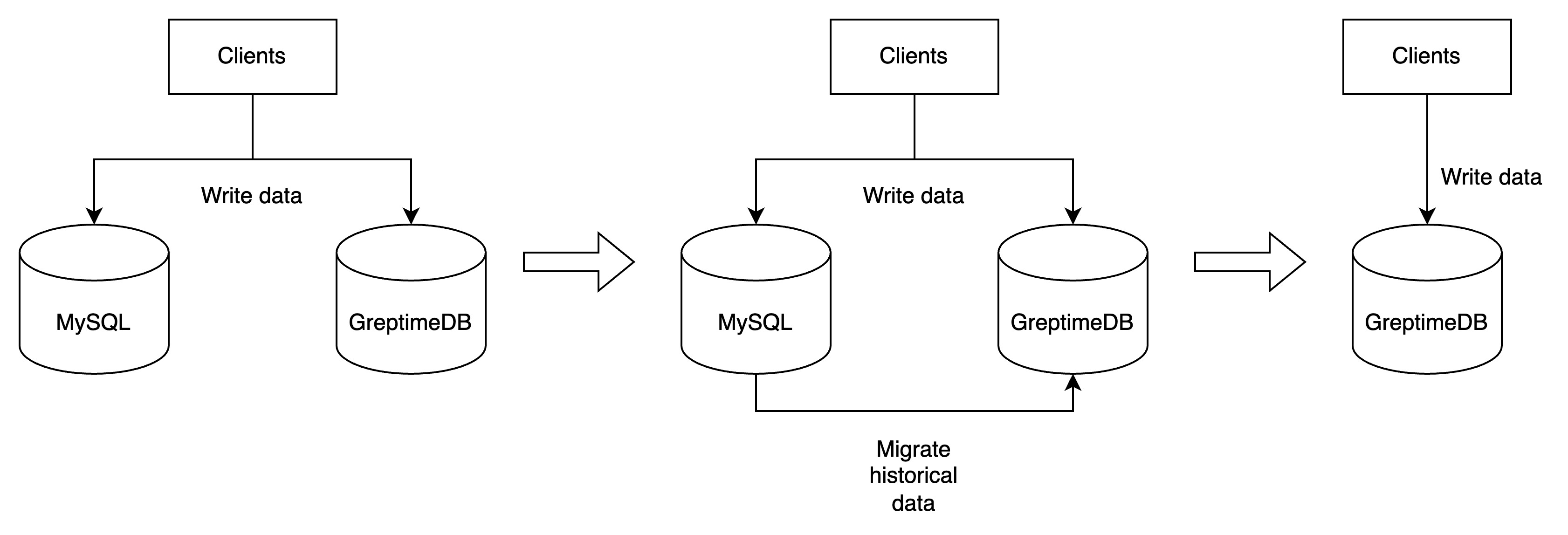
After the data migration is completed, you can stop writing data to MySQL and continue using GreptimeDB exclusively!
If you need a more detailed migration plan or example scripts, please provide the specific table structure and data volume. The [GreptimeDB official community](https://github.com/orgs/GreptimeTeam/discussions) will offer further support. Welcome to join the [Greptime Slack](http://greptime.com/slack).
---
## Migrate from PostgreSQL
This document will guide you through the migration process from PostgreSQL to GreptimeDB.
## Before you start the migration
Please be aware that though GreptimeDB supports the wire protocol of PostgreSQL, it does not mean GreptimeDB implements
all
PostgreSQL's features. You may refer to:
* The [ANSI Compatibility](/reference/sql/compatibility.md) to see the constraints regarding using SQL in GreptimeDB.
* The [Data Modeling Guide](/user-guide/deployments-administration/performance-tuning/design-table.md) to create proper table schemas.
* The [Data Index Guide](/user-guide/manage-data/data-index.md) for index planning.
## Migration steps
### Create the databases and tables in GreptimeDB
Before migrating the data from PostgreSQL, you first need to create the corresponding databases and tables in
GreptimeDB.
GreptimeDB has its own SQL syntax for creating tables, so you cannot directly reuse the table creation SQLs that are
produced
by PostgreSQL.
When you write the table creation SQL for GreptimeDB, it's important to understand
its "[data model](/user-guide/concepts/data-model.md)" first. Then, please take the following considerations in
your create table SQL:
1. Since the time index column cannot be changed after the table is created, you need to choose the time index column
carefully. The time index is best set to the natural timestamp when the data is generated, as it provides the most
intuitive way to query the data, and the best query performance. For example, in the IOT scenes, you can use the
collection time of sensor data as the time index; or the occurrence time of an event in the observability scenes.
2. In this migration process, it's not recommend to create another synthetic timestamp, such as a new column created
with `DEFAULT current_timestamp()` as the time index column. It's not recommend to use the random timestamp as the
time index either.
3. It's vital to set the most fit timestamp precision for your time index column, too. Like the chosen of time index
column, the precision of it cannot be changed as well. Find the most fit timestamp type for your
data set [here](/reference/sql/data-types#data-types-compatible-with-mysql-and-postgresql).
4. Choose a primary key only when it is truly needed. The primary key in GreptimeDB is different from that in PostgreSQL. You should use a primary key only when:
* Most queries can benefit from the ordering.
* You need to deduplicate (including delete) rows by the primary key and time index.
Otherwise, setting a primary key is optional and it may hurt performance. Read [Primary Key](/user-guide/deployments-administration/performance-tuning/design-table.md#primary-key) for details.
Finally please refer to "[CREATE](/reference/sql/create.md)" SQL document for more details for choosing the
right data types and "ttl" or "compaction" options, etc.
5. Choose proper indexes to speed up queries.
* Inverted index: is ideal for filtering by low-cardinality columns and quickly finding rows with specific values.
* Skipping index: works well with sparse data.
* Fulltext index: enables efficient keyword and pattern search in large text columns.
For details and best practices, refer to the [data index](user-guide/manage-data/data-index.md) documentation.
### Write data to both GreptimeDB and PostgreSQL simultaneously
Writing data to both GreptimeDB and PostgreSQL simultaneously is a practical strategy to avoid data loss during
migration. By utilizing PostgreSQL's client libraries (JDBC + a PostgreSQL driver), you can set up two client
instances - one for GreptimeDB and another for PostgreSQL. For guidance on writing data to GreptimeDB using SQL, please
refer to the [Ingest Data](/user-guide/ingest-data/for-iot/sql.md) section.
If retaining all historical data isn't necessary, you can simultaneously write data to both GreptimeDB and PostgreSQL
for a specific period to accumulate the required recent data. Subsequently, cease writing to PostgreSQL and continue
exclusively with GreptimeDB. If a complete migration of all historical data is needed, please proceed with the following
steps.
### Export data from PostgreSQL
[pg_dump](https://www.postgresql.org/docs/current/app-pgdump.html) is a commonly used tool to export data from
PostgreSQL. Using it, we can export the data that can be later imported into GreptimeDB directly. For example, if we
want to export schemas whose names start with `db` in the database `postgres` from PostgreSQL, we can use the following
command:
```bash
pg_dump -h127.0.0.1 -p5432 -Upostgres -ax --column-inserts --no-comments -n 'db*' postgres | grep -v "^SE" > /path/to/output.sql
```
Replace the `-h`, `-p` and `-U` flags with the appropriate values for your PostgreSQL server. The `-n` flag is used to
specify the schemas to be exported. And the database `postgres` is at the end of the `pg_dump` command line. Note that we pipe the `pg_dump` output through a special
`grep`, to remove some unnecessary `SET` or `SELECT` lines. The final output will be written to the
`/path/to/output.sql` file.
The content in the `/path/to/output.sql` file should be like this:
```plaintext
~ ❯ cat /path/to/output.sql
--
-- PostgreSQL database dump
--
-- Dumped from database version 16.4 (Debian 16.4-1.pgdg120+1)
-- Dumped by pg_dump version 16.4
--
-- Data for Name: foo; Type: TABLE DATA; Schema: db1; Owner: postgres
--
INSERT INTO db1.foo (ts, a) VALUES ('2024-10-31 00:00:00', 1);
INSERT INTO db1.foo (ts, a) VALUES ('2024-10-31 00:00:01', 2);
INSERT INTO db1.foo (ts, a) VALUES ('2024-10-31 00:00:01', 3);
INSERT INTO ...
--
-- Data for Name: foo; Type: TABLE DATA; Schema: db2; Owner: postgres
--
INSERT INTO db2.foo (ts, b) VALUES ('2024-10-31 00:00:00', '1');
INSERT INTO db2.foo (ts, b) VALUES ('2024-10-31 00:00:01', '2');
INSERT INTO db2.foo (ts, b) VALUES ('2024-10-31 00:00:01', '3');
INSERT INTO ...
--
-- PostgreSQL database dump complete
--
```
### Import data into GreptimeDB
The [psql -- PostgreSQL interactive terminal](https://www.postgresql.org/docs/current/app-psql.html) can be used to
we can use the following command to import the data into GreptimeDB:
```bash
psql -h127.0.0.1 -p4003 -d public -f /path/to/output.sql
```
Replace the `-h` and `-p` flags with the appropriate values for your GreptimeDB server. The `-d` of the psql command is used to specify the database and cannot be omitted. The value `public` of `-d` is the default database used by GreptimeDB. You can also add `-a` to the end to see every
executed line, or `-s` for entering the single-step mode.
To summarize, data migration steps can be illustrate as follows:

After the data migration is completed, you can stop writing data to PostgreSQL and continue using GreptimeDB
exclusively!
If you need a more detailed migration plan or example scripts, please provide the specific table structure and data volume. The [GreptimeDB official community](https://github.com/orgs/GreptimeTeam/discussions) will offer further support. Welcome to join the [Greptime Slack](http://greptime.com/slack).
---
## Migrate from Prometheus
For information on configuring Prometheus to write data to GreptimeDB, please refer to the [remote write](/user-guide/ingest-data/for-observability/prometheus.md#remote-write-configuration) documentation.
For detailed information on querying data in GreptimeDB using Prometheus query language, please refer to the [HTTP API](/user-guide/query-data/promql.md#prometheus-http-api) section in the PromQL documentation.
To add GreptimeDB as a Prometheus data source in Grafana, please refer to the [Grafana](/user-guide/integrations/grafana.md#prometheus-data-source) documentation.
---
## Migrate to GreptimeDB
You can migrate data from various databases to GreptimeDB,
including InfluxDB, MySQL, PostgreSQL, Prometheus, and more.
---
## User Guide
Welcome to the user guide for GreptimeDB.
GreptimeDB is the unified observability database for metrics, logs, and traces,
providing real-time insights from Edge to Cloud at any scale.
## Understanding GreptimeDB Concepts
Before diving into GreptimeDB,
it is recommended to familiarize yourself with its data model, key concepts, and features.
For a comprehensive overview,
refer to the [Concepts Documentation](./concepts/overview.md).
## Ingesting Data Based on Your Use Case
GreptimeDB supports [multiple protocols](./protocols/overview.md) and [various integration tools](./integrations/overview.md) to simplify data ingestion tailored to your requirements.
### For Observability Scenarios
If you plan to use GreptimeDB as metrics, logs and traces storage for observability purposes,
see the [Observability Documentation](./ingest-data/for-observability/overview.md).
It explains how to ingest data using tools like Otel-Collector, Vector, Kafka, Prometheus, and the InfluxDB line protocol.
For a log storage solution,
refer to the [Logs Documentation](./logs/overview.md).
It details how to ingest pattern text logs using pipelines.
For a trace storage solution,
refer to the [Traces Documentation](./traces/overview.md).
It explains how to ingest trace data using OpenTelemetry and query it with Jaeger.
### For IoT and Edge Computing Scenarios
For IoT and Edge Computing scenarios,
the [IoT Documentation](./ingest-data/for-iot/overview.md) provides comprehensive guidance on ingesting data from diverse sources.
## Querying Data for Insights
GreptimeDB offers robust interfaces for [querying data](./query-data/overview.md).
### SQL Support
You can use SQL for range queries, aggregations, and more.
For detailed instructions, see the [SQL Query Documentation](./query-data/sql.md).
### Prometheus Query Language (PromQL)
GreptimeDB supports PromQL for querying data. Refer to the [PromQL Documentation](./query-data/promql.md) for guidance.
### Flow Computation
For real-time data processing and analysis, GreptimeDB provides [Flow Computation](./flow-computation/overview.md), enabling complex computations on data streams.
## Accelerating Queries with Indexes
Indexes such as inverted indexes, skipping indexes, and full-text indexes can significantly enhance query performance.
Learn more about effectively using these indexes in the [Data Index Documentation](./manage-data/data-index.md).
## Migrating to GreptimeDB from Other Databases
Migrating data from other databases to GreptimeDB is straightforward.
Follow the step-by-step instructions in the [Migration Documentation](./migrate-to-greptimedb/overview.md).
## Administering and Deploying GreptimeDB
When you're ready to deploy GreptimeDB, consult the [Deployment & Administration Documentation](/user-guide/deployments-administration/overview.md) for detailed guidance on deployment and management.
---
## Elasticsearch(Protocols)
Please refer to [Ingest Data with Elasticsearch](/user-guide/ingest-data/for-observability/elasticsearch.md) for detailed information.
---
## gRPC
GreptimeDB offers [gRPC SDKs](/user-guide/ingest-data/for-iot/grpc-sdks/overview.md) for efficient and high-performance data ingestion.
If there is no SDK available for your programming language, you have the option to [create your own SDK](/contributor-guide/how-to/how-to-write-sdk.md) by following the guidelines provided in the contributor guide.
---
## HTTP API
GreptimeDB provides HTTP APIs for interacting with the database. For a complete list of available APIs, please refer to the [HTTP Endpoint](/reference/http-endpoints.md).
## Base URL
The base URL of API is `http(s)://{{host}}:{{port}}/`.
- For the GreptimeDB instance running on the local machine,
with default port configuration `4000`,
the base URL is `http://localhost:4000/`.
You can change the server host and port in the [configuration](/user-guide/deployments-administration/configuration.md#protocol-options) file.
- For GreptimeCloud, the base URL is `https://{{host}}/`.
You can find the host in 'Connection Information' at the GreptimeCloud console.
In the following sections, we use `http://{{API-host}}/` as the base URL to demonstrate the API usage.
## Common headers
### Authentication
Assume that you have already configured the database [authentication](/user-guide/deployments-administration/authentication/overview.md) correctly,
GreptimeDB supports the built-in `Basic` authentication scheme in the HTTP API. To set up authentication, follow these steps:
1. Encode your username and password using the `:` format and the `Base64` algorithm.
2. Attach your encoded credentials to the one of the following HTTP header:
- `Authorization: Basic `
- `x-greptime-auth: Basic `
Here's an example. If you want to connect to GreptimeDB using the username `greptime_user` and password `greptime_pwd`, use the following command:
```shell
curl -X POST \
-H 'Authorization: Basic Z3JlcHRpbWVfdXNlcjpncmVwdGltZV9wd2Q=' \
-H 'Content-Type: application/x-www-form-urlencoded' \
-d 'sql=show tables' \
http://localhost:4000/v1/sql
```
In this example, `Z3JlcHRpbWVfdXNlcjpncmVwdGltZV9wd2Q=` represents the Base64-encoded value of `greptime_user:greptime_pwd`. Make sure to replace it with your own configured username and password, and encode them using Base64.
:::tip NOTE
InfluxDB uses its own authentication format, see [InfluxDB](./influxdb-line-protocol.md) for details.
:::
### Timeout
GreptimeDB supports the `X-Greptime-Timeout` header in HTTP requests.
It is used to specify the timeout for the request running in the database server.
For example, the following request set `120s` timeout for the request:
```bash
curl -X POST \
-H 'Authorization: Basic {{authentication}}' \
-H 'X-Greptime-Timeout: 120s' \
-H 'Content-Type: application/x-www-form-urlencoded' \
-d 'sql=show tables' \
http://localhost:4000/v1/sql
```
### Hints
GreptimeDB supports the `x-greptime-hints` header in HTTP requests to pass hint key-value pairs that influence request behavior.
These hints are primarily used to set table options when tables are [automatically created](/user-guide/ingest-data/overview.md#automatic-schema-generation) during data ingestion.
The format is a comma-separated list of `key=value` pairs:
```
x-greptime-hints: key1=value1, key2=value2
```
Supported hints:
| Hint | Type | Default | Description |
| --- | --- | --- | --- |
| `auto_create_table` | Boolean | `true` | Whether to automatically create the table if it does not exist when inserting data. |
| `ttl` | Duration string | None | Sets the [time-to-live](/user-guide/manage-data/overview.md#manage-data-retention-with-ttl-policies) for the table, e.g. `7d`, `24h`. Expired data will be automatically purged. |
| `append_mode` | Boolean | `false` | Enables [append-only mode](/reference/sql/create.md#create-an-append-only-table) for the table, which disables deduplication by primary key and supports duplicate rows. |
| `merge_mode` | String | None | Sets the [merge mode](/reference/sql/create.md#create-a-table-with-merge-mode) for the table, e.g. `last_non_null`, `last_row`. |
| `physical_table` | String | None | Specifies the physical table name for the [metric engine](/contributor-guide/datanode/metric-engine.md). |
| `skip_wal` | Boolean | `false` | Skips WAL (Write-Ahead Log) writes for the table. |
| `sst_format` | String | None | Sets the SST (Sorted String Table) file format for the table. Valid values: `flat`, `primary_key`. |
For example, the following request sets TTL and append mode for auto-created tables:
```bash
curl -X POST \
-H 'Authorization: Basic {{authentication}}' \
-H 'x-greptime-hints: ttl=7d, append_mode=true' \
-H 'Content-Type: application/x-www-form-urlencoded' \
-d 'sql=INSERT INTO my_table VALUES (...)' \
http://localhost:4000/v1/sql
```
## Admin APIs
:::tip NOTE
These endpoint cannot be used in GreptimeCloud.
:::
Please refer to the [Admin APIs](/reference/http-endpoints.md#admin-apis) documentation for more information.
## POST SQL statements
To submit a SQL query to the GreptimeDB server via HTTP API, use the following format:
```shell
curl -X POST \
-H 'Authorization: Basic {{authentication}}' \
-H 'X-Greptime-Timeout: {{timeout}}' \
-H 'Content-Type: application/x-www-form-urlencoded' \
-d 'sql={{SQL-statement}}' \
http://{{API-host}}/v1/sql
```
### Headers
- [`Authorization`](#authentication)
- [`X-Greptime-Timeout`](#timeout)
- `Content-Type`: `application/x-www-form-urlencoded`.
- `X-Greptime-Timezone`: The time zone for the current SQL query. Optional. Please refer to [time zone](#time-zone).
### Query string parameters
- `db`: The database name. Optional. If not provided, the default database `public` will be used.
- `format`: The output format. Optional. `greptimedb_v1` by default.
In addition to the default JSON format, the HTTP API also allows you to
customize output format by providing the `format` query parameter with following
values:
- `influxdb_v1`: [influxdb query
API](https://docs.influxdata.com/influxdb/v1/tools/api/#query-http-endpoint)
compatible format. Additional parameters:
- `epoch`: `[ns,u,µ,ms,s,m,h]`, returns epoch timestamps with the specified
precision
- `csv`: outputs as comma-separated values
- `csvWithNames`: outputs as comma-separated values with a column names header
- `csvWithNamesAndTypes`: outputs as comma-separated values with column names and data types headers
- `arrow`: [Arrow IPC
format](https://arrow.apache.org/docs/python/feather.html). We use stream
format for this API. Additional
parameters:
- `compression`: `zstd` or `lz4`, default: no compression
- `table`: ASCII table format for console output
- `null`: Concise text-only output of the row count and elapsed time, useful for evaluating query performance.
### Body
- `sql`: The SQL statement. Required.
### Response
The response is a JSON object containing the following fields:
- `output`: The SQL executed result. Please refer to the examples below to see the details.
- `execution_time_ms`: The execution time of the statement in milliseconds.
### Examples
#### `INSERT` statement
For example, to insert data into the `monitor` table of database `public`, use the following command:
```shell
curl -X POST \
-H 'Authorization: Basic {{authorization if exists}}' \
-H 'Content-Type: application/x-www-form-urlencoded' \
-d 'sql=INSERT INTO monitor VALUES ("127.0.0.1", 1667446797450, 0.1, 0.4), ("127.0.0.2", 1667446798450, 0.2, 0.3), ("127.0.0.1", 1667446798450, 0.5, 0.2)' \
http://localhost:4000/v1/sql?db=public
```
The response will contain the number of affected rows:
```shell
{"output":[{"affectedrows":3}],"execution_time_ms":11}
```
#### `SELECT` statement
You can also use the HTTP API to execute other SQL statements.
For example, to retrieve data from the `monitor` table:
```shell
curl -X POST \
-H 'Authorization: Basic {{authorization if exists}}' \
-H 'Content-Type: application/x-www-form-urlencoded' \
-d "sql=SELECT * FROM monitor" \
http://localhost:4000/v1/sql?db=public
```
The response will contain the queried data in JSON format:
```json
{
"output": [
{
"records": {
"schema": {
"column_schemas": [
{
"name": "host",
"data_type": "String"
},
{
"name": "ts",
"data_type": "TimestampMillisecond"
},
{
"name": "cpu",
"data_type": "Float64"
},
{
"name": "memory",
"data_type": "Float64"
}
]
},
"rows": [
[
"127.0.0.1",
1720728000000,
0.5,
0.1
]
],
"total_rows": 1
}
}
],
"execution_time_ms": 7
}
```
The response contains the following fields:
- `output`: The execution result.
- `records`: The query result.
- `schema`: The schema of the result, including the schema of each column.
- `rows`: The rows of the query result, where each row is an array containing the corresponding values of the columns in the schema.
- `execution_time_ms`: The execution time of the statement in milliseconds.
#### Time zone
GreptimeDB supports the `X-Greptime-Timezone` header in HTTP requests.
It is used to specify the timezone for the current SQL query.
For example, the following request uses the time zone `+1:00` for the query:
```bash
curl -X POST \
-H 'Authorization: Basic {{authentication}}' \
-H 'X-Greptime-Timezone: +1:00' \
-H 'Content-Type: application/x-www-form-urlencoded' \
-d 'sql=SHOW VARIABLES time_zone;' \
http://localhost:4000/v1/sql
```
After the query, the result will be:
```json
{
"output": [
{
"records": {
"schema": {
"column_schemas": [
{
"name": "TIME_ZONE",
"data_type": "String"
}
]
},
"rows": [
[
"+01:00"
]
]
}
}
],
"execution_time_ms": 27
}
```
For information on how the time zone affects data inserts and queries, please refer to the SQL documents in the [Ingest Data](../ingest-data/for-iot/sql.md#time-zone) and [Query Data](../query-data/sql.md#time-zone) sections.
#### Query data with `table` format output
You can use the `table` format in the query string parameters to get the output in ASCII table format.
```shell
curl -X POST \
-H 'Authorization: Basic {{authorization if exists}}' \
-H 'Content-Type: application/x-www-form-urlencoded' \
-d "sql=SELECT * FROM monitor" \
http://localhost:4000/v1/sql?db=public&format=table
```
Output
```
┌─host────────┬─ts────────────┬─cpu─┬─memory─┐
│ "127.0.0.1" │ 1667446797450 │ 0.1 │ 0.4 │
│ "127.0.0.1" │ 1667446798450 │ 0.5 │ 0.2 │
│ "127.0.0.2" │ 1667446798450 │ 0.2 │ 0.3 │
└─────────────┴───────────────┴─────┴────────┘
```
#### Query data with `csvWithNames` format output
```shell
curl -X POST \
-H 'Authorization: Basic {{authorization if exists}}' \
-H 'Content-Type: application/x-www-form-urlencoded' \
-d "sql=SELECT * FROM monitor" \
http://localhost:4000/v1/sql?db=public&format=csvWithNames
```
Output:
```csv
host,ts,cpu,memory
127.0.0.1,1667446797450,0.1,0.4
127.0.0.1,1667446798450,0.5,0.2
127.0.0.2,1667446798450,0.2,0.3
```
Changes `format` to `csvWithNamesAndTypes`:
```shell
curl -X POST \
-H 'Authorization: Basic {{authorization if exists}}' \
-H 'Content-Type: application/x-www-form-urlencoded' \
-d "sql=SELECT * FROM monitor" \
http://localhost:4000/v1/sql?db=public&format=csvWithNamesAndTypes
```
Output:
```csv
host,ts,cpu,memory
String,TimestampMillisecond,Float64,Float64
127.0.0.1,1667446797450,0.1,0.4
127.0.0.1,1667446798450,0.5,0.2
127.0.0.2,1667446798450,0.2,0.3
```
#### Query data with `influxdb_v1` format output
You can use the `influxdb_v1` format in the query string parameters to get the output in InfluxDB query API compatible format.
```shell
curl -X POST \
-H 'Authorization: Basic {{authorization if exists}}' \
-H 'Content-Type: application/x-www-form-urlencoded' \
-d "sql=SELECT * FROM monitor" \
http://localhost:4000/v1/sql?db=public&format=influxdb_v1&epoch=ms
```
```json
{
"results": [
{
"statement_id": 0,
"series": [
{
"name": "",
"columns": [
"host",
"ts",
"cpu",
"memory"
],
"values": [
["127.0.0.1", 1667446797450, 0.1, 0.4],
["127.0.0.1", 1667446798450, 0.5, 0.2],
["127.0.0.2", 1667446798450, 0.2, 0.3]
]
}
]
}
],
"execution_time_ms": 2
}
```
### Parse SQL with GreptimeDB's SQL dialect
To parse and understand queries written in GreptimeDB's SQL dialect for tools like dashboards, etc., you can use the `/v1/sql/parse` endpoint to obtain the structured result of an SQL query:
```shell
curl -X POST \
-H 'Authorization: Basic {{authorization if exists}}' \
-H 'Content-Type: application/x-www-form-urlencoded' \
-d "sql=SELECT * FROM monitor" \
http://localhost:4000/v1/sql/parse
```
```json
[
{
"Query": {
"inner": {
"with": null,
"body": {
"Select": {
"select_token": {
"token": {
"Word": {
"value": "SELECT",
"quote_style": null,
"keyword": "SELECT"
}
},
"span": {
"start": {
"line": 1,
"column": 1
},
"end": {
"line": 1,
"column": 7
}
}
},
"optimizer_hint": null,
"distinct": null,
"select_modifiers": null,
"top": null,
"top_before_distinct": false,
"projection": [
{
"Wildcard": {
"wildcard_token": {
"token": "Mul",
"span": {
"start": {
"line": 1,
"column": 8
},
"end": {
"line": 1,
"column": 9
}
}
},
"opt_ilike": null,
"opt_exclude": null,
"opt_except": null,
"opt_replace": null,
"opt_rename": null
}
}
],
"exclude": null,
"into": null,
"from": [
{
"relation": {
"Table": {
"name": [
{
"Identifier": {
"value": "monitor",
"quote_style": null,
"span": {
"start": {
"line": 1,
"column": 15
},
"end": {
"line": 1,
"column": 22
}
}
}
}
],
"alias": null,
"args": null,
"with_hints": [],
"version": null,
"with_ordinality": false,
"partitions": [],
"json_path": null,
"sample": null,
"index_hints": []
}
},
"joins": []
}
],
"lateral_views": [],
"prewhere": null,
"selection": null,
"connect_by": [],
"group_by": {
"Expressions": [
[],
[]
]
},
"cluster_by": [],
"distribute_by": [],
"sort_by": [],
"having": null,
"named_window": [],
"qualify": null,
"window_before_qualify": false,
"value_table_mode": null,
"flavor": "Standard"
}
},
"order_by": null,
"limit_clause": null,
"fetch": null,
"locks": [],
"for_clause": null,
"settings": null,
"format_clause": null,
"pipe_operators": []
},
"hybrid_cte": null
}
}
]
```
## POST PromQL queries
### The API returns Prometheus query result format
GreptimeDB compatible with Prometheus query language (PromQL) and can be used to query data in GreptimeDB.
For all the compatible APIs, please refer to the [Prometheus Query Language](/user-guide/query-data/promql#prometheus-http-api) documentation.
### The API returns GreptimeDB JSON format
GreptimeDB also exposes an custom HTTP API for querying with PromQL, and returning
GreptimeDB's data frame output. You can find it on `/promql` path under the
current stable API version `/v1`.
The return value of this API is in GreptimeDB's JSON format, not Prometheus's format.
For example:
```shell
curl -X GET \
-H 'Authorization: Basic {{authorization if exists}}' \
-G \
--data-urlencode 'query=avg(system_metrics{idc="idc_a"})' \
--data-urlencode 'start=1667446797' \
--data-urlencode 'end=1667446799' \
--data-urlencode 'step=1s' \
'http://localhost:4000/v1/promql?db=public'
```
The input parameters are similar to the [`range_query`](https://prometheus.io/docs/prometheus/latest/querying/api/#range-queries) in Prometheus' HTTP API:
- `db=`: Required when using GreptimeDB with authorization, otherwise can be omitted if you are using the default `public` database. Note this parameter should be set in the query param, or using a HTTP header `--header 'x-greptime-db-name: '`.
- `query=`: Required. Prometheus expression query string.
- `start=`: Required. The start timestamp, which is inclusive. It is used to set the range of time in `TIME INDEX` column.
- `end=`: Required. The end timestamp, which is inclusive. It is used to set the range of time in `TIME INDEX` column.
- `step=`: Required. Query resolution step width in duration format or float number of seconds.
- `format`: The output format. Optional. `greptimedb_v1` by default.
In addition to the default JSON format, the HTTP API also allows you to
customize output format by providing the `format` query parameter with following
values:
- `influxdb_v1`: [influxdb query
API](https://docs.influxdata.com/influxdb/v1/tools/api/#query-http-endpoint)
compatible format. Additional parameters:
- `epoch`: `[ns,u,µ,ms,s,m,h]`, returns epoch timestamps with the specified
precision
- `csv`: outputs as comma-separated values
- `csvWithNames`: outputs as comma-separated values with a column names header
- `csvWithNamesAndTypes`: outputs as comma-separated values with column names and data types headers
- `arrow`: [Arrow IPC
format](https://arrow.apache.org/docs/python/feather.html). Additional
parameters:
- `compression`: `zstd` or `lz4`, default: no compression
- `table`: ASCII table format for console output
- `null`: Concise text-only output of the row count and elapsed time, useful for evaluating query performance.
Here are some examples for each type of parameter:
- rfc3339
- `2015-07-01T20:11:00Z` (default to seconds resolution)
- `2015-07-01T20:11:00.781Z` (with milliseconds resolution)
- `2015-07-02T04:11:00+08:00` (with timezone offset)
- unix timestamp
- `1435781460` (default to seconds resolution)
- `1435781460.781` (with milliseconds resolution)
- duration
- `1h` (1 hour)
- `5d1m` (5 days and 1 minute)
- `2` (2 seconds)
- `2s` (also 2 seconds)
The result format is the same as `/sql` interface described in [Post SQL statements](#post-sql-statements) section.
```json
{
"output": [
{
"records": {
"schema": {
"column_schemas": [
{
"name": "ts",
"data_type": "TimestampMillisecond"
},
{
"name": "AVG(system_metrics.cpu_util)",
"data_type": "Float64"
},
{
"name": "AVG(system_metrics.memory_util)",
"data_type": "Float64"
},
{
"name": "AVG(system_metrics.disk_util)",
"data_type": "Float64"
}
]
},
"rows": [
[
1667446798000,
80.1,
70.3,
90
],
[
1667446799000,
80.1,
70.3,
90
]
]
}
}
],
"execution_time_ms": 5
}
```
## Post Influxdb line protocol data
```shell
curl -X POST \
-H 'Authorization: token {{username:password}}' \
-d '{{Influxdb-line-protocol-data}}' \
http://{{API-host}}/v1/influxdb/api/v2/write?precision={{time-precision}}
```
```shell
curl -X POST \
-d '{{Influxdb-line-protocol-data}}' \
http://{{API-host}}/v1/influxdb/write?u={{username}}&p={{password}}&precision={{time-precision}}
```
### Headers
- `Authorization`: **Unlike other APIs**, the InfluxDB line protocol APIs use the InfluxDB authentication format. For V2, it is `token {{username:password}}`.
### Query string parameters
- `u`: The username. Optional. It is the authentication username for V1.
- `p`: The password. Optional. It is the authentication password for V1.
- `db`: The database name. Optional. The default value is `public`.
- `precision`: Defines the precision of the timestamp provided in the request body. Please refer to [InfluxDB Line Protocol](/user-guide/ingest-data/for-iot/influxdb-line-protocol.md) in the user guide.
### Body
The InfluxDB line protocol data points. Please refer to the [InfluxDB Line Protocol](https://docs.influxdata.com/influxdb/v1/write_protocols/line_protocol_tutorial/#syntax) document.
### Examples
Please refer to [InfluxDB Line Protocol](/user-guide/ingest-data/for-iot/influxdb-line-protocol.md) in the user guide.
## API for managing Pipelines
When writing logs to GreptimeDB,
you can use HTTP APIs to manage the pipelines.
For detailed information,
please refer to the [Manage Pipelines](/user-guide/logs/manage-pipelines.md) documentation.
---
## InfluxDB Line Protocol(Protocols)
## Ingest data
For how to ingest data to GreptimeDB using InfluxDB Line Protocol,
please refer to the [Ingest Data](/user-guide/ingest-data/for-iot/influxdb-line-protocol.md) document.
## HTTP API
Please refer to the [HTTP API](http.md#post-influxdb-line-protocol-data) document for details on the InfluxDB Line Protocol API.
## PING
Additionally, GreptimeDB also provides support for the `ping` and `health` APIs of InfluxDB.
Use `curl` to request `ping` API.
```shell
curl -i "127.0.0.1:4000/v1/influxdb/ping"
```
```shell
HTTP/1.1 204 No Content
date: Wed, 22 Feb 2023 02:29:44 GMT
```
Use `curl` to request `health` API.
```shell
curl -i "127.0.0.1:4000/v1/influxdb/health"
```
```shell
HTTP/1.1 200 OK
content-length: 0
date: Wed, 22 Feb 2023 02:30:46 GMT
```
---
## Loki(Protocols)
Please refer to [Ingest Data with Loki](/user-guide/ingest-data/for-observability/loki.md) for detailed information.
---
## MySQL
## Connect
You can connect to GreptimeDB using MySQL via port `4002`.
```shell
mysql -h -P 4002 -u -p
```
- For how to setup username and password for GreptimeDB, please refer to [Authentication](/user-guide/deployments-administration/authentication/overview.md).
- If you want to use other ports for MySQL, please refer to [Protocol options](/user-guide/deployments-administration/configuration.md#protocol-options) in the configuration document.
## Table management
Please refer to [Table Management](/user-guide/deployments-administration/manage-data/basic-table-operations.md).
## Ingest data
Please refer to [SQL](/user-guide/ingest-data/for-iot/sql.md).
## Query data
Please refer to [SQL](/user-guide/query-data/sql.md).
## Time zone
GreptimeDB's MySQL protocol interface follows original MySQL on [how to
deal with time zone](https://dev.mysql.com/doc/refman/8.0/en/time-zone-support.html).
By default, MySQL uses its server time zone for timestamp. To override, you can
set `time_zone` variable for current session using SQL statement `SET time_zone = '';`.
The value of `time_zone` can be any of:
- The server's time zone: `SYSTEM`.
- Offset to UTC such as `+08:00`.
- Any named time zone like `Europe/Berlin`.
Some MySQL clients, such as Grafana MySQL data source, allow you to set the time zone for the current session.
You can also use the above values when setting the time zone.
You can use `SELECT` to check the current time zone settings. For example:
```sql
SELECT @@system_time_zone, @@time_zone;
```
The result shows that both the system time zone and the session time zone are set to `UTC`:
```SQL
+--------------------+-------------+
| @@system_time_zone | @@time_zone |
+--------------------+-------------+
| UTC | UTC |
+--------------------+-------------+
```
Change the session time zone to `+1:00`:
```SQL
SET time_zone = '+1:00'
```
Then you can see the difference between the system time zone and the session time zone:
```SQL
SELECT @@system_time_zone, @@time_zone;
+--------------------+-------------+
| @@system_time_zone | @@time_zone |
+--------------------+-------------+
| UTC | +01:00 |
+--------------------+-------------+
```
For information on how the time zone affects data inserts and queries, please refer to the SQL documents in the [Ingest Data](/user-guide/ingest-data/for-iot/sql.md#time-zone) and [Query Data](/user-guide/query-data/sql.md#time-zone) sections.
## Query Timeout
You can set the `max_execution_time` variable for the current session using SQL statement `SET max_execution_time = ` or `SET MAX_EXECUTION_TIME = `, which specifies the maximum time in milliseconds for a **read-only statement** to execute. The server will terminate the query if it exceeds the specified time.
For example, to set the maximum query execution time to 10 seconds:
```SQL
SET max_execution_time=10000;
```
---
## OpenTelemetry (OTLP)
GreptimeDB is an observability backend to consume OpenTelemetry Metrics natively via [OTLP/HTTP](https://opentelemetry.io/docs/specs/otlp/#otlphttp) protocol.
Please refer to the [Ingest Data with OpenTelemetry](/user-guide/ingest-data/for-observability/opentelemetry.md) document for detailed information.
---
## OpenTSDB(Protocols)
Please refer to [Ingest Data with OpenTSDB](/user-guide/ingest-data/for-iot/opentsdb.md) for detailed information.
---
## Protocols
---
## PostgreSQL
## Connect
You can connect to GreptimeDB using PostgreSQL via port `4003`.
Simply add the `-U` argument to your command, followed by your username and password. Here's an example:
```shell
psql -h -p 4003 -U -d public
```
- For how to setup username and password for GreptimeDB, please refer to [Authentication](/user-guide/deployments-administration/authentication/overview.md).
- If you want to use other ports for PostgreSQL, please refer to [Protocol options](/user-guide/deployments-administration/configuration.md#protocol-options) in the configuration document.
## Table management
Please refer to [Table Management](/user-guide/deployments-administration/manage-data/basic-table-operations.md).
## Ingest data
Please refer to [SQL](/user-guide/ingest-data/for-iot/sql.md).
## Query data
Please refer to [SQL](/user-guide/query-data/sql.md).
## Time zone
GreptimeDB's PostgreSQL protocol interface follows original PostgreSQL on [datatype-timezones](https://www.postgresql.org/docs/current/datatype-datetime.html#DATATYPE-TIMEZONES).
By default, PostgreSQL uses its server time zone for timestamp. To override, you can
set `time_zone` variable for current session using SQL statement `SET TIMEZONE TO '';`.
The value of `time_zone` can be any of:
- A full time zone name, for example `America/New_York`.
- A time zone abbreviation, for example `PST`.
- Offset to UTC such as `+08:00`.
You can use `SHOW` to check the current time zone settings. For example:
```sql
SHOW VARIABLES time_zone;
```
```sql
TIME_ZONE
-----------
UTC
```
Change the session time zone to `+1:00`:
```SQL
SET TIMEZONE TO '+1:00'
```
For information on how the time zone affects data inserts and queries, please refer to the SQL documents in the [Ingest Data](/user-guide/ingest-data/for-iot/sql.md#time-zone) and [Query Data](/user-guide/query-data/sql.md#time-zone) sections.
## Foreign Data Wrapper
GreptimeDB can be configured as a foreign data server for Postgres' built-in
[FDW extension](https://www.postgresql.org/docs/current/postgres-fdw.html). This
allows user to query GreptimeDB tables seamlessly from Postgres server. It's
also possible to join Postgres tables with GreptimeDB tables.
For example, your IoT metadata, like device information, is stored in a
relational data model in Postgres. It's possible to use filter queries to find
out device IDs and join with time-series data from GreptimeDB.
### Setup
To setup GreptimeDB for Postgres FDW, make sure you enabled postgres protocol
support in GreptimeDB and it's accessible from your Postgres server.
To create and configuration GreptimeDB in Postgres, first enable the
`postgres_fdw` extension.
```sql
CREATE EXTENSION postgres_fdw;
```
Add GreptimeDB instance as remote server.
```sql
CREATE SERVER greptimedb
FOREIGN DATA WRAPPER postgres_fdw
OPTIONS (host 'greptimedb_host', dbname 'public', port '4003');
```
Configure user mapping for Postgres user and GreptimeDB user. This step is
required. But if you don't have authentication enabled in GreptimeDB OSS
version, just fill the credential with random data.
```sql
CREATE USER MAPPING FOR postgres
SERVER greptimedb
OPTIONS (user 'greptime', password '...');
```
Create foreign table in Postgres to map GreptimeDB's schema. Note that you will
need to use Postgres' corresponding data types for GreptimeDB's.
For GreptimeDB's tables
```sql
CREATE TABLE grpc_latencies (
ts TIMESTAMP TIME INDEX,
host STRING,
method_name STRING,
latency DOUBLE,
PRIMARY KEY (host, method_name)
) with('append_mode'='true');
CREATE TABLE app_logs (
ts TIMESTAMP TIME INDEX,
host STRING,
api_path STRING FULLTEXT INDEX,
log_level STRING,
log STRING FULLTEXT INDEX,
PRIMARY KEY (host, log_level)
) with('append_mode'='true');
```
The foreign table DDL is like this. You need to run them in Postgres to create
these tables;
```sql
CREATE FOREIGN TABLE ft_grpc_latencies (
ts TIMESTAMP,
host VARCHAR,
method_name VARCHAR,
latency DOUBLE precision
)
SERVER greptimedb
OPTIONS (table_name 'grpc_latencies');
CREATE FOREIGN TABLE ft_app_logs (
ts TIMESTAMP,
host VARCHAR,
api_path VARCHAR,
log_level VARCHAR,
log VARCHAR
)
SERVER greptimedb
OPTIONS (table_name 'app_logs');
```
To help you to generate statements in Postgres, we enhanced `SHOW CREATE TABLE`
in GreptimeDB to dump the Postgres DDL for you. For example:
```sql
SHOW CREATE TABLE grpc_latencies FOR postgres_foreign_table;
```
Note that you will need to replace server name `greptimedb` with the name you
defined in `CREATE SERVER` statement.
### Run Queries
You can now send query from Postgres. It's also possible to use functions that
are available in both Postgres and GreptimeDB, like `date_trunc`.
```sql
SELECT * FROM ft_app_logs ORDER BY ts DESC LIMIT 100;
SELECT
date_trunc('MINUTE', ts) as t,
host,
avg(latency),
count(latency)
FROM ft_grpc_latencies GROUP BY host, t;
```
## Statement Timeout
You can set the `statement_timeout` variable for the current session using SQL statement `SET statement_timeout = ` or `SET STATEMENT_TIMEOUT = `, which specifies the maximum time in milliseconds for a statement to execute. The server will terminate the statement if it exceeds the specified time.
For example, to set the maximum execution time to 10 seconds:
```SQL
SET statement_timeout=10000;
```
---
## Common Table Expression (CTE)
CTEs are similar to [Views](./view.md) in that they help you reduce the complexity of your queries, break down long and complex SQL statements, and improve readability and reusability.
You already read a CTE in the [quickstart](/getting-started/quick-start.md#correlate-metrics-logs-and-traces) document.
## What is a Common Table Expression (CTE)?
A Common Table Expression (CTE) is a temporary result set that you can reference within a `SELECT`, `INSERT`, `UPDATE`, or `DELETE` statement. CTEs help to break down complex queries into more readable parts and can be referenced multiple times within the same query.
## Basic syntax of CTE
CTEs are typically defined using the `WITH` keyword. The basic syntax is as follows:
```sql
WITH cte_name [(column1, column2, ...)] AS (
QUERY
)
SELECT ...
FROM cte_name;
```
## Example explanation
Next, we'll go through a complete example that demonstrates how to use CTEs, including data preparation, CTE creation, and usage.
### Step 1: Create example data
Let's assume we have the following two tables:
- `grpc_latencies`: Contains gRPC request latency data.
- `app_logs`: Contains application log information.
```sql
CREATE TABLE grpc_latencies (
ts TIMESTAMP TIME INDEX,
host VARCHAR(255),
latency FLOAT,
PRIMARY KEY(host),
);
INSERT INTO grpc_latencies VALUES
('2023-10-01 10:00:00', 'host1', 120),
('2023-10-01 10:00:00', 'host2', 150),
('2023-10-01 10:00:05', 'host1', 130);
CREATE TABLE app_logs (
ts TIMESTAMP TIME INDEX,
host VARCHAR(255),
`log` TEXT,
log_level VARCHAR(50),
PRIMARY KEY(host, log_level),
);
INSERT INTO app_logs VALUES
('2023-10-01 10:00:00', 'host1', 'Error on service', 'ERROR'),
('2023-10-01 10:00:00', 'host2', 'All services OK', 'INFO'),
('2023-10-01 10:00:05', 'host1', 'Error connecting to DB', 'ERROR');
```
### Step 2: Define and use CTEs
We will create two CTEs to calculate the 95th percentile latency and the number of error logs, respectively.
```sql
WITH
metrics AS (
SELECT
ts,
host,
approx_percentile_cont(0.95) WITHIN GROUP (ORDER BY latency) RANGE '5s' AS p95_latency
FROM
grpc_latencies
ALIGN '5s' FILL PREV
),
logs AS (
SELECT
ts,
host,
COUNT(*) RANGE '5s' AS num_errors
FROM
app_logs
WHERE
log_level = 'ERROR'
ALIGN '5s' BY (host)
)
SELECT
metrics.ts,
metrics.host,
metrics.p95_latency,
COALESCE(logs.num_errors, 0) AS num_errors
FROM
metrics
LEFT JOIN logs ON metrics.host = logs.host AND metrics.ts = logs.ts
ORDER BY
metrics.ts;
```
Output:
```sql
+---------------------+-------+-------------+------------+
| ts | host | p95_latency | num_errors |
+---------------------+-------+-------------+------------+
| 2023-10-01 10:00:00 | host2 | 150 | 0 |
| 2023-10-01 10:00:00 | host1 | 120 | 1 |
| 2023-10-01 10:00:05 | host1 | 130 | 1 |
+---------------------+-------+-------------+------------+
```
## Detailed explanation
1. **Define CTEs**:
- `metrics`:
```sql
WITH
metrics AS (
SELECT
ts,
host,
approx_percentile_cont(0.95) WITHIN GROUP (ORDER BY latency) RANGE '5s' AS p95_latency
FROM
grpc_latencies
ALIGN '5s' FILL PREV
),
```
Here we use a [range query](/user-guide/query-data/sql.md#aggregate-data-by-time-window) to calculate the 95th percentile latency for each `host` within every 5-second window.
- `logs`:
```sql
logs AS (
SELECT
ts,
host,
COUNT(*) RANGE '5s' AS num_errors
FROM
app_logs
WHERE
log_level = 'ERROR'
ALIGN '5s' BY (host)
)
```
Similarly, we calculate the number of error logs for each `host` within every 5-second window.
2. **Use CTEs**:
The final query part:
```sql
SELECT
metrics.ts,
metrics.host,
metrics.p95_latency,
COALESCE(logs.num_errors, 0) AS num_errors
FROM
metrics
LEFT JOIN logs ON metrics.host = logs.host AND metrics.ts = logs.ts
ORDER BY
metrics.ts;
```
We perform a left join on the two CTE result sets to get a comprehensive analysis result.
## Using TQL in CTEs
GreptimeDB supports using [TQL](/reference/sql/tql.md) (Telemetry Query Language) within CTEs, allowing you to combine PromQL's time-series computation with SQL's powerful post-processing capabilities like filtering, joining, and aggregation.
### Basic syntax
```sql
WITH cte_name AS (
TQL EVAL (start, end, step) promql_expression AS value_alias
)
SELECT * FROM cte_name;
```
### Key points
1. **Column naming**:
- The time index column name varies depending on your table schema (e.g., `ts` for custom tables, `greptime_timestamp` for Prometheus remote write)
- The value column name depends on the PromQL expression and may be unpredictable, so it's better to use value aliasing with `AS` in TQL to ensure predictable column names: `TQL EVAL (...) expression AS my_value`
- **Important**: In general, avoid using column aliases in CTE definitions (for example, `WITH cte_name (ts, val) AS (...)`) because TQL EVAL results can have variable column count and order, especially in Prometheus scenarios where tags can be dynamically added or removed. They are best reserved for cases where the result shape is stable, such as a simple `CREATE FLOW` TQL CTE.
2. **Supported commands**: Only `TQL EVAL` is supported within CTEs. `TQL ANALYZE` and `TQL EXPLAIN` cannot be used in CTEs.
3. **Lookback parameter**: The optional fourth parameter controls the lookback duration (default: 5 minutes).
4. **Using TQL CTEs in `CREATE FLOW`**: GreptimeDB supports `WITH ... AS (TQL EVAL ...)` in `CREATE FLOW`, but only in the simplest form: a single TQL CTE followed by `SELECT * FROM `. Extra SQL CTEs, filters, joins, or custom projections are not supported in flow definitions.
### Examples
The following examples use Kubernetes monitoring metrics to demonstrate practical use cases.
#### Filtering TQL results with SQL
This example calculates CPU usage per pod using PromQL, then filters and sorts the results using SQL:
```sql
WITH cpu_usage AS (
TQL EVAL (now() - interval '1' hour, now(), '5m')
sum by (namespace, pod) (rate(container_cpu_usage_seconds_total{container!=""}[5m]))
AS cpu_cores
)
SELECT
greptime_timestamp as ts,
namespace,
pod,
cpu_cores
FROM cpu_usage
WHERE cpu_cores > 0.5
ORDER BY cpu_cores DESC;
```
#### Correlating multiple metrics
This example demonstrates a capability that PromQL alone cannot achieve: joining different metrics for correlation analysis. It correlates CPU usage with request rates to analyze resource efficiency:
```sql
WITH
cpu_data AS (
TQL EVAL (now() - interval '1' hour, now(), '5m')
sum by (pod) (rate(container_cpu_usage_seconds_total{container!=""}[5m]))
AS cpu_cores
),
request_data AS (
TQL EVAL (now() - interval '1' hour, now(), '5m')
sum by (pod) (rate(http_requests_total[5m]))
AS req_per_sec
)
SELECT
c.greptime_timestamp as ts,
c.pod,
c.cpu_cores,
r.req_per_sec
FROM cpu_data c
JOIN request_data r
ON c.greptime_timestamp = r.greptime_timestamp
AND c.pod = r.pod
WHERE r.req_per_sec > 1;
```
When joining multiple TQL CTEs, ensure:
- The `by (...)` clauses contain matching dimensions
- JOIN conditions include both timestamp and label columns
## Summary
With CTEs, you can break down complex SQL queries into more manageable and understandable parts. In this example, we created two CTEs to calculate the 95th percentile latency and the number of error logs separately and then merged them into the final query for analysis. TQL support in CTEs extends this capability by allowing PromQL-style queries to be integrated seamlessly with SQL processing. Read more about [WITH](/reference/sql/with.md) and [TQL](/reference/sql/tql.md).
For more TQL + CTE examples, see the blog post [When PromQL Meets SQL: Hybrid Queries for Kubernetes Monitoring](https://greptime.com/blogs/2026-01-08-tql-alias-k8s-monitoring).
---
## Jaeger (Experimental)
:::warning
The Jaeger query APIs are currently in the experimental stage and may be adjusted in future versions.
:::
GreptimeDB currently supports the following [Jaeger](https://www.jaegertracing.io/) query interfaces:
- `/api/services`: Get all services.
- `/api/operations?service={service}`: Get all operations for a service.
- `/api/services/{service}/operations`: Get all operations for a service.
- `/api/traces`: Get traces by query parameters.
You can use [Grafana's Jaeger plugin](https://grafana.com/docs/grafana/latest/datasources/jaeger/)(Recommended) or [Jaeger UI](https://github.com/jaegertracing/jaeger-ui) to query traces data in GreptimeDB. When using Jaeger UI, you can set the `proxyConfig` in `packages/jaeger-ui/vite.config.mts` to the GreptimeDB address, for example:
```ts
const proxyConfig = {
target: 'http://localhost:4000/v1/jaeger',
secure: false,
changeOrigin: true,
ws: true,
xfwd: true,
};
```
Currently, GreptimeDB exposes the Jaeger HTTP APIs under the `/v1/jaeger` endpoint.
## Quick Start
We will use the Jaeger plugin in Grafana as an example to demonstrate how to query traces data in GreptimeDB. Before starting, please ensure that you have properly started GreptimeDB.
### Start an application to generate traces data and write it to GreptimeDB
You can refer to the [OpenTelemetry official documentation](https://opentelemetry.io/docs/languages/) to choose any programming language you are familiar with to generate traces data. You can also refer to the [Configure OpenTelemetry Collector](/user-guide/traces/read-write.md#opentelemetry-collector) document.
### Configure the Grafana Jaeger plugin
1. Open Grafana and add a Jaeger data source:
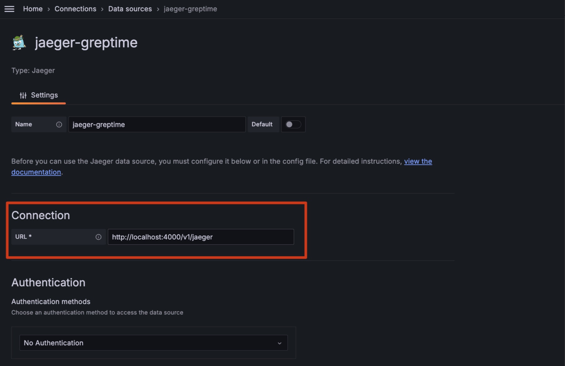
2. Fill in the Jaeger address according to your actual situation, then **Save and Test**. For example:
```
http://localhost:4000/v1/jaeger
```
3. Use Grafana's Jaeger Explore to view the data:
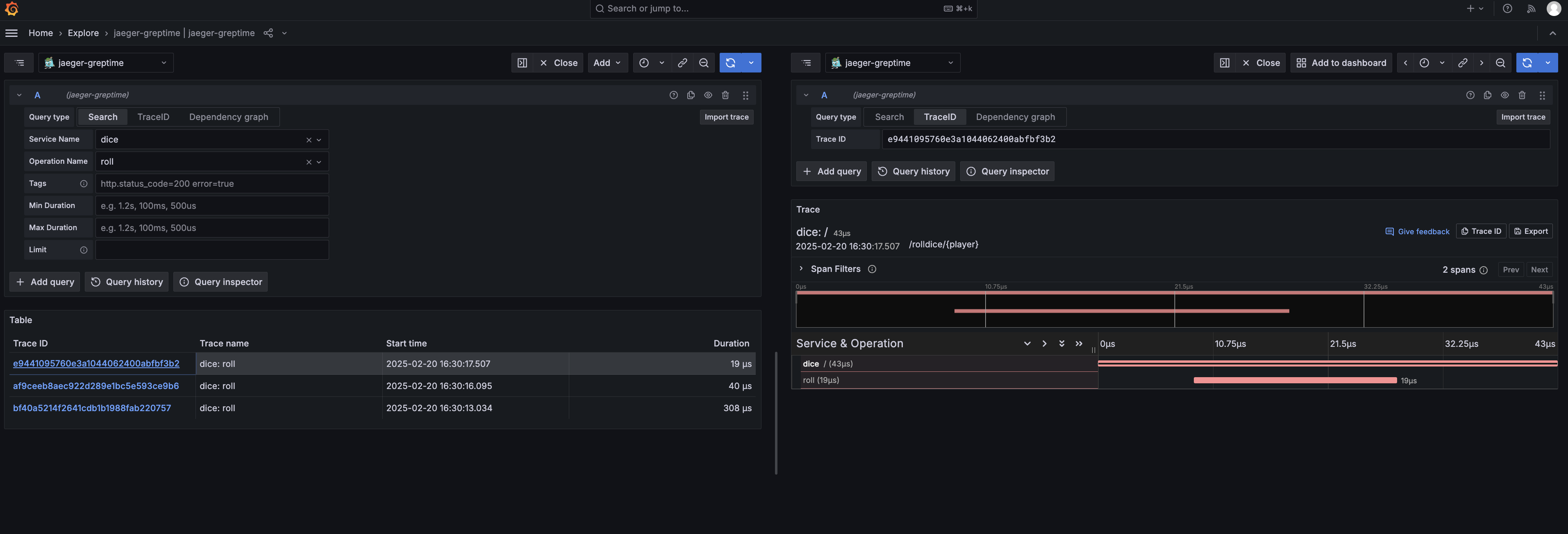
### Custom table
By default, the jaeger compatible API will use the default table name
`opentelemetry_traces` for its data. If you have multiple tables for trace data,
you can update this behaviour with HTTP header `x-greptime-trace-table-name` and
provide table name as the value.
This can be configured via Grafana data source settings.
---
## Log Query (Experimental)
:::warning
The log query endpoint feature is currently experimental and may change in future releases.
:::
GreptimeDB provides a dedicated HTTP endpoint to query log data. This feature allows you to search and process log entries using a simple query interface. This is an add-on feature to existing GreptimeDB capabilities like SQL queries and Flow computations. You can still use your existing tools and workflows to query log data like before.
## Endpoint
```http
POST /v1/logs
```
## Headers
- [Authorization](/user-guide/protocols/http.md#authentication)
- `Content-Type`: `application/json`
## Request Format
The request body should be a JSON object (this is subject to change in patch version within the experimental phase). For the latest request format, please refer to the [implementation](https://github.com/GreptimeTeam/greptimedb/blob/main/src/log-query/src/log_query.rs):
## Response
This endpoint has the same response format as the SQL query endpoint. Please refer to the [SQL query response](/user-guide/protocols/http/#response) for more details.
## Limitations
- Maximum result limit: 1000 entries
- Only supports tables with timestamp and string columns
## Example
The following example demonstrates how to query log data using the log query endpoint (notice that in this experimental phase the following example might be outdated).
```shell
curl -X "POST" "http://localhost:4000/v1/logs" \
-H "Authorization: Basic {{authentication}}" \
-H "Content-Type: application/json" \
-d $'
{
"table": {
"catalog_name": "greptime",
"schema_name": "public",
"table_name": "my_logs"
},
"time_filter": {
"start": "2025-01-23"
},
"limit": {
"fetch": 1
},
"columns": [
"message"
],
"filters": [
{
"column_name": "message",
"filters": [
{
"Contains": "production"
}
]
}
],
"context": "None",
"exprs": []
}
'
```
In this query, we are searching for log entries in the `greptime.public.my_logs` table that contain the word `production` in `message` field. We also specify the time filter to fetch logs in `2025-01-23`, and limit the result to 1 entry.
The response will be similar to the following:
```json
{
"output": [
{
"records": {
"schema": {
"column_schemas": [
{
"name": "message",
"data_type": "String"
}
]
},
"rows": [
[
"Everything is in production"
]
],
"total_rows": 1
}
}
],
"execution_time_ms": 30
}
```
---
## Query Data
## Query languages
- [PromQL](./promql.md)
- [SQL](./sql.md)
- [Log Query](./log-query.md) (Experimental)
Since v0.9, GreptimeDB supports view and CTE just like other databases, used to simplify queries:
* [View](./view.md)
* [Common Table Expression (CTE)](./cte.md)
## Recommended libraries
Since GreptimeDB uses SQL as its main query language and supports both [MySQL](/user-guide/protocols/mysql.md) and [PostgreSQL](/user-guide/protocols/postgresql.md) protocols,
you can use mature SQL drivers that support MySQL or PostgreSQL to query data.
For more information, please refer to the [SQL Tools](/reference/sql-tools.md) documentation.
## Query external data
GreptimeDB has the capability to query external data files. For more information, please refer to the [Query External Data](./query-external-data.md) documentation.
---
## Prometheus Query Language
GreptimeDB can be used as a drop-in replacement for Prometheus in Grafana, because GreptimeDB supports PromQL (Prometheus Query Language). GreptimeDB has reimplemented PromQL natively in Rust and exposes the ability to several interfaces, including the HTTP API of Prometheus, the HTTP API of GreptimeDB, and the SQL interface.
## Prometheus' HTTP API
GreptimeDB has implemented a set of Prometheus compatible APIs under HTTP
context `/v1/prometheus/`:
- Instant queries `/api/v1/query`
- Range queries `/api/v1/query_range`
- Series `/api/v1/series`
- Label names `/api/v1/labels`
- Label values `/api/v1/label//values`
It shares same input and output format with original Prometheus HTTP API. You
can also use GreptimeDB as an in-place replacement of Prometheus. For example in
Grafana Prometheus data source, set `http://localhost:4000/v1/prometheus/` as
context root of Prometheus URL.
Consult [Prometheus
documents](https://prometheus.io/docs/prometheus/latest/querying/api) for usage
of these API.
You can use additional query parameter `db` to specify GreptimeDB database name.
For example, the following query will return the CPU usage of the `process_cpu_seconds_total` metric in the `public` database:
```shell
curl -X POST \
-H 'Authorization: Basic {{authorization if exists}}' \
--data-urlencode 'query=irate(process_cpu_seconds_total[1h])' \
--data-urlencode 'start=2024-11-24T00:00:00Z' \
--data-urlencode 'end=2024-11-25T00:00:00Z' \
--data-urlencode 'step=1h' \
'http://localhost:4000/v1/prometheus/api/v1/query_range?db=public'
```
If authentication is enabled in GreptimeDB, the authentication header is required. Refer to the [authentication documentation](/user-guide/protocols/http.md#authentication) for more details.
You need to either set it in the HTTP URL query param `db` like the example above, or set it using `--header 'x-greptime-db-name: '` as HTTP header.
The query string parameters for the API are identical to those of the original [Prometheus API](https://prometheus.io/docs/prometheus/latest/querying/api/#range-queries), with the exception of the additional `db` parameter, which specifies the GreptimeDB database name.
The output format is compatible with the Prometheus API:
```json
{
"status": "success",
"data": {
"resultType": "matrix",
"result": [
{
"metric": {
"job": "node",
"instance": "node_exporter:9100",
"__name__": "process_cpu_seconds_total"
},
"values": [
[
1732618800,
"0.0022222222222222734"
],
[
1732622400,
"0.0009999999999999788"
],
[
1732626000,
"0.0029999999999997585"
],
[
1732629600,
"0.002222222222222175"
]
]
}
]
}
}
```
## SQL
GreptimeDB also extends SQL grammar to support PromQL. You can start with the `TQL` (Time-series Query Language) keyword to write parameters and queries. The grammar looks like this:
```sql
TQL [EVAL|EVALUATE] (, , )
```
`` specifies the query start range and `` specifies the end time. `` identifies the query resolution step width. All of them can either be an unquoted number (represent UNIX timestamp for `` and ``, and duration in seconds for ``), or a quoted string (represent an RFC3339 timestamp for `` and ``, and duration in string format for ``).
For example:
```sql
TQL EVAL (1676738180, 1676738780, '10s') sum(some_metric)
```
You can write the above command in all places that support SQL, including the GreptimeDB HTTP API, SDK, PostgreSQL and MySQL client etc.
## GreptimeDB's extensions to PromQL
### Specifying value field
Based on the table model, GreptimeDB supports multiple fields in a single table(or metric, in the context of Prometheus). Queries will run on every fields by default. Or you can use the special filter `__field__` to query a specific field(s):
```promql
metric{__field__="field1"}
```
Exclude or regex are also supported:
```promql
metric{__field__!="field1"}
metric{__field__=~"field_1|field_2"}
metric{__field__!~"field_1|field_2"}
```
### Cross-database query
Greptime has its own database concept. In order to run cross-database query, you
can use `__database__` matcher to specify the database name.
```promql
metric{__database__="mydatabase"}
```
Note that only `=` is supported for database matcher.
## Limitations
Though GreptimeDB supports a rich set of data types, the PromQL implementation is still limited to the following types:
- timestamp: `Timestamp`
- tag: `String`
- value: `Double`
We have over 90% promql supported in GreptimeDB. Here attaches the compatibility list. You can also check our latest compliance report in this [tracking issue](https://github.com/GreptimeTeam/greptimedb/issues/1042).
### Literal
Both string and float literals are supported, with the same [rule](https://prometheus.io/docs/prometheus/latest/querying/basics/#literals) as PromQL.
### Selector
Both instant and range selector are supported. But notice that in both Prometheus and GreptimeDB, the label matching on metric name is an exception. Negative matching (e.g. `{__name__!="request_count}"`) is not allowed. Others like equal-matching or regex-matching are supported.
Time duration and offset are supported, but `@` modifier is not supported yet.
When selecting non-existent columns, they will be treated as columns filled with empty string values (`""`). This behavior aligns with both Prometheus and VictoriaMetrics.
For selectors referencing non-existent columns, the behavior aligns with Prometheus: no error is raised, and the selector is silently ignored. However, for `__name__` selectors referencing non-existent metrics (or equivalent forms), GreptimeDB will report an error.
### Timestamp precision
The timestamp precision in PromQL is limited by its query syntax, only supporting calculations up to millisecond precision. However, GreptimeDB supports storing high-precision timestamps, such as microseconds and nanoseconds. When using PromQL for calculations, these high-precision timestamps are implicitly converted to millisecond precision.
### Binary
- Supported:
| Operator |
| :------- |
| add |
| sub |
| mul |
| div |
| mod |
| eqlc |
| neq |
| gtr |
| lss |
| gte |
| lte |
| power |
| atan2 |
| and |
| or |
| unless |
- Unsupported:
None
### Aggregators
- Supported:
| Aggregator | Example |
| :----------- | :------------------------------------------- |
| sum | `sum by (foo)(metric)` |
| avg | `avg by (foo)(metric)` |
| min | `min by (foo)(metric)` |
| max | `max by (foo)(metric)` |
| stddev | `stddev by (foo)(metric)` |
| stdvar | `stdvar by (foo)(metric)` |
| topk | `topk(3, rate(instance_cpu_time_ns[5m]))` |
| bottomk | `bottomk(3, rate(instance_cpu_time_ns[5m]))` |
| count_values | `count_values("version", build_version)` |
| count | `count (metric)` |
| quantile | `quantile(0.9, cpu_usage)` |
- Unsupported:
| Aggregator | Progress |
| :--------- | :------- |
| grouping | TBD |
### Instant Functions
- Supported:
| Function | Example |
| :----------------- | :-------------------------------- |
| abs | `abs(metric)` |
| ceil | `ceil(metric)` |
| exp | `exp(metric)` |
| ln | `ln(metric)` |
| log2 | `log2(metric)` |
| log10 | `log10(metric)` |
| sqrt | `sqrt(metric)` |
| acos | `acos(metric)` |
| asin | `asin(metric)` |
| atan | `atan(metric)` |
| sin | `sin(metric)` |
| cos | `cos(metric)` |
| tan | `tan(metric)` |
| acosh | `acosh(metric)` |
| asinh | `asinh(metric)` |
| atanh | `atanh(metric)` |
| sinh | `sinh(metric)` |
| cosh | `cosh(metric)` |
| scalar | `scalar(metric)` |
| tanh | `tanh(metric)` |
| timestamp | `timestamp()` |
| sort | `sort(http_requests_total)` |
| sort_desc | `sort_desc(http_requests_total)` |
| histogram_quantile | `histogram_quantile(phi, metric)` |
| predicate_linear | `predict_linear(metric, 120)` |
| absent | `absent(nonexistent{job="myjob"})`|
| sgn | `sgn(metric)` |
| pi | `pi()` |
| deg | `deg(metric)` |
| rad | `rad(metric)` |
| floor | `floor(metric)` |
| clamp | `clamp(metric, 0, 12)` |
| clamp_max | `clamp_max(metric, 12)` |
| clamp_min | `clamp_min(metric, 0)` |
- Unsupported:
| Function | Progress / Example |
| :------------------------- | :----------------- |
| *other multiple input fns* | TBD |
### Range Functions
- Supported:
| Function | Example |
| :----------------- | :----------------------------- |
| idelta | `idelta(metric[5m])` |
| \_over_time | `count_over_time(metric[5m])` |
| stddev_over_time | `stddev_over_time(metric[5m])` |
| stdvar_over_time | `stdvar_over_time(metric[5m])` |
| changes | `changes(metric[5m])` |
| delta | `delta(metric[5m])` |
| rate | `rate(metric[5m])` |
| deriv | `deriv(metric[5m])` |
| increase | `increase(metric[5m])` |
| irate | `irate(metric[5m])` |
| reset | `reset(metric[5m])` |
- Unsupported:
None
### Label & Other Functions
- Supported:
| Function | Example |
| :------------ | :------------------------------------------------------------------------------------------------ |
| label_join | `label_join(up{job="api-server",src1="a",src2="b",src3="c"}, "foo", ",", "src1", "src2", "src3")` |
| label_replace | `label_replace(up{job="api-server",service="a:c"}, "foo", "$1", "service", "(.*):.*")` |
| sort_by_label | `sort_by_label(metric, "foo", "bar")` |
| sort_by_label_desc | `sort_by_label_desc(metric, "foo", "bar")` |
- Unsupported:
None
---
## Query External Data
## Query on a file
Currently, we support queries on `Parquet`, `CSV`, `ORC`, and `NDJson` format file(s).
We use the [Taxi Zone Lookup Table](https://d37ci6vzurychx.cloudfront.net/misc/taxi+_zone_lookup.csv) data as an example.
```bash
curl "https://d37ci6vzurychx.cloudfront.net/misc/taxi+_zone_lookup.csv" -o /tmp/taxi+_zone_lookup.csv
```
Create an external table:
```sql
CREATE EXTERNAL TABLE taxi_zone_lookup with (location='/tmp/taxi+_zone_lookup.csv',format='csv');
```
You can check the schema of the external table like follows:
```sql
DESC TABLE taxi_zone_lookup;
```
```sql
+--------------------+----------------------+------+------+--------------------------+---------------+
| Column | Type | Key | Null | Default | Semantic Type |
+--------------------+----------------------+------+------+--------------------------+---------------+
| LocationID | Int64 | | YES | | FIELD |
| Borough | String | | YES | | FIELD |
| Zone | String | | YES | | FIELD |
| service_zone | String | | YES | | FIELD |
| greptime_timestamp | TimestampMillisecond | PRI | NO | 1970-01-01 00:00:00+0000 | TIMESTAMP |
+--------------------+----------------------+------+------+--------------------------+---------------+
4 rows in set (0.00 sec)
```
:::tip Note
Here, you may notice there is a `greptime_timestamp` column, which doesn't exist in the file. This is because when creating an external table, if we didn't specify a `TIME INDEX` column, the `greptime_timestamp` column is automatically added as the `TIME INDEX` column with a default value of `1970-01-01 00:00:00+0000`. You can find more details in the [create](/reference/sql/create.md#create-external-table) document.
:::
Now you can query on the external table:
```sql
SELECT `Zone`, `Borough` FROM taxi_zone_lookup LIMIT 5;
```
```sql
+-------------------------+---------------+
| Zone | Borough |
+-------------------------+---------------+
| Newark Airport | EWR |
| Jamaica Bay | Queens |
| Allerton/Pelham Gardens | Bronx |
| Alphabet City | Manhattan |
| Arden Heights | Staten Island |
+-------------------------+---------------+
```
## Query on a directory
Let's download some data:
```bash
mkdir /tmp/external
curl "https://d37ci6vzurychx.cloudfront.net/trip-data/yellow_tripdata_2022-01.parquet" -o /tmp/external/yellow_tripdata_2022-01.parquet
curl "https://d37ci6vzurychx.cloudfront.net/trip-data/yellow_tripdata_2022-02.parquet" -o /tmp/external/yellow_tripdata_2022-02.parquet
```
Verify the download:
```bash
ls -l /tmp/external
total 165368
-rw-r--r-- 1 wenyxu wheel 38139949 Apr 28 14:35 yellow_tripdata_2022-01.parquet
-rw-r--r-- 1 wenyxu wheel 45616512 Apr 28 14:36 yellow_tripdata_2022-02.parquet
```
Create the external table:
```sql
CREATE EXTERNAL TABLE yellow_tripdata with(location='/tmp/external/',format='parquet');
```
Run queries:
```sql
SELECT count(*) FROM yellow_tripdata;
```
```sql
+-----------------+
| COUNT(UInt8(1)) |
+-----------------+
| 5443362 |
+-----------------+
1 row in set (0.48 sec)
```
```sql
SELECT * FROM yellow_tripdata LIMIT 5;
```
```sql
+----------+----------------------+-----------------------+-----------------+---------------+------------+--------------------+--------------+--------------+--------------+-------------+-------+---------+------------+--------------+-----------------------+--------------+----------------------+-------------+---------------------+
| VendorID | tpep_pickup_datetime | tpep_dropoff_datetime | passenger_count | trip_distance | RatecodeID | store_and_fwd_flag | PULocationID | DOLocationID | payment_type | fare_amount | extra | mta_tax | tip_amount | tolls_amount | improvement_surcharge | total_amount | congestion_surcharge | airport_fee | greptime_timestamp |
+----------+----------------------+-----------------------+-----------------+---------------+------------+--------------------+--------------+--------------+--------------+-------------+-------+---------+------------+--------------+-----------------------+--------------+----------------------+-------------+---------------------+
| 1 | 2022-02-01 00:06:58 | 2022-02-01 00:19:24 | 1 | 5.4 | 1 | N | 138 | 252 | 1 | 17 | 1.75 | 0.5 | 3.9 | 0 | 0.3 | 23.45 | 0 | 1.25 | 1970-01-01 00:00:00 |
| 1 | 2022-02-01 00:38:22 | 2022-02-01 00:55:55 | 1 | 6.4 | 1 | N | 138 | 41 | 2 | 21 | 1.75 | 0.5 | 0 | 6.55 | 0.3 | 30.1 | 0 | 1.25 | 1970-01-01 00:00:00 |
| 1 | 2022-02-01 00:03:20 | 2022-02-01 00:26:59 | 1 | 12.5 | 1 | N | 138 | 200 | 2 | 35.5 | 1.75 | 0.5 | 0 | 6.55 | 0.3 | 44.6 | 0 | 1.25 | 1970-01-01 00:00:00 |
| 2 | 2022-02-01 00:08:00 | 2022-02-01 00:28:05 | 1 | 9.88 | 1 | N | 239 | 200 | 2 | 28 | 0.5 | 0.5 | 0 | 3 | 0.3 | 34.8 | 2.5 | 0 | 1970-01-01 00:00:00 |
| 2 | 2022-02-01 00:06:48 | 2022-02-01 00:33:07 | 1 | 12.16 | 1 | N | 138 | 125 | 1 | 35.5 | 0.5 | 0.5 | 8.11 | 0 | 0.3 | 48.66 | 2.5 | 1.25 | 1970-01-01 00:00:00 |
+----------+----------------------+-----------------------+-----------------+---------------+------------+--------------------+--------------+--------------+--------------+-------------+-------+---------+------------+--------------+-----------------------+--------------+----------------------+-------------+---------------------+
5 rows in set (0.11 sec)
```
:::tip Note
The query result includes the value of the `greptime_timestamp` column, although it does not exist in the original file. All these column values are `1970-01-01 00:00:00+0000`, because when we create an external table, the `greptime_timestamp` column is automatically added with a default value of `1970-01-01 00:00:00+0000`. You can find more details in the [create](/reference/sql/create.md#create-external-table) document.
:::
---
## SQL(Query-data)
GreptimeDB supports full SQL for querying data from a database.
In this document, we will use the `monitor` table to demonstrate how to query data.
For instructions on creating the `monitor` table and inserting data into it,
Please refer to [table management](/user-guide/deployments-administration/manage-data/basic-table-operations.md#create-a-table) and [Ingest Data](/user-guide/ingest-data/for-iot/sql.md).
## Basic query
The query is represented by the `SELECT` statement.
For example, the following query selects all data from the `monitor` table:
```sql
SELECT * FROM monitor;
```
The query result looks like the following:
```sql
+-----------+---------------------+------+--------+
| host | ts | cpu | memory |
+-----------+---------------------+------+--------+
| 127.0.0.1 | 2022-11-03 03:39:57 | 0.1 | 0.4 |
| 127.0.0.1 | 2022-11-03 03:39:58 | 0.5 | 0.2 |
| 127.0.0.2 | 2022-11-03 03:39:58 | 0.2 | 0.3 |
+-----------+---------------------+------+--------+
3 rows in set (0.00 sec)
```
Functions are also supported in the `SELECT` field list.
For example, you can use the `count()` function to retrieve the total number of rows in the table:
```sql
SELECT count(*) FROM monitor;
```
```sql
+-----------------+
| COUNT(UInt8(1)) |
+-----------------+
| 3 |
+-----------------+
```
The `avg()` function returns the average value of a certain field:
```sql
SELECT avg(cpu) FROM monitor;
```
```sql
+---------------------+
| AVG(monitor.cpu) |
+---------------------+
| 0.26666666666666666 |
+---------------------+
1 row in set (0.00 sec)
```
You can also select only the result of a function.
For example, you can extract the day of the year from a timestamp.
The `DOY` in the SQL statement is the abbreviation of `day of the year`:
```sql
SELECT date_part('DOY', '2021-07-01 00:00:00');
```
Output:
```sql
+----------------------------------------------------+
| date_part(Utf8("DOY"),Utf8("2021-07-01 00:00:00")) |
+----------------------------------------------------+
| 182 |
+----------------------------------------------------+
1 row in set (0.003 sec)
```
The parameters and results of date functions align with the SQL client's time zone.
For example, when the client's time zone is set to `+08:00`, the results of the two queries below are the same:
```sql
select to_unixtime('2024-01-02 00:00:00');
select to_unixtime('2024-01-02 00:00:00+08:00');
```
Please refer to [SELECT](/reference/sql/select.md) and [Functions](/reference/sql/functions/overview.md) for more information.
## Limit the number of rows returned
Time series data is typically massive.
To save bandwidth and improve query performance,
you can use the `LIMIT` clause to restrict the number of rows returned by the `SELECT` statement.
For example, the following query limits the number of rows returned to 10:
```sql
SELECT * FROM monitor LIMIT 10;
```
## Filter data
You can use the `WHERE` clause to filter the rows returned by the `SELECT` statement.
Filtering data by tags or time index is efficient and common in time series scenarios.
For example, the following query filter data by tag `host`:
```sql
SELECT * FROM monitor WHERE host='127.0.0.1';
```
The following query filter data by time index `ts`, and returns the data after `2022-11-03 03:39:57`:
```sql
SELECT * FROM monitor WHERE ts > '2022-11-03 03:39:57';
```
You can also use the `AND` keyword to combine multiple constraints:
```sql
SELECT * FROM monitor WHERE host='127.0.0.1' AND ts > '2022-11-03 03:39:57';
```
### Filter by time index
Filtering data by the time index is a crucial feature in time series databases.
When working with Unix time values, the database treats them based on the type of the column value.
For instance, if the `ts` column in the `monitor` table has a value type of `TimestampMillisecond`,
you can use the following query to filter the data:
The Unix time value `1667446797000` corresponds to the `TimestampMillisecond` type。
```sql
SELECT * FROM monitor WHERE ts > 1667446797000;
```
When working with a Unix time value that doesn't have the precision of the column value,
you need to use the `::` syntax to specify the type of the time value.
This ensures that the database correctly identifies the type.
For example, `1667446797` represents a timestamp in seconds,
which is different from the default millisecond timestamp of the `ts` column.
You need to specify its type as `TimestampSecond` using the `::TimestampSecond` syntax.
This informs the database that the value `1667446797` should be treated as a timestamp in seconds.
```sql
SELECT * FROM monitor WHERE ts > 1667446797::TimestampSecond;
```
For the supported time data types, please refer to [Data Types](/reference/sql/data-types.md#date-and-time-types).
When using standard `RFC3339` or `ISO8601` string literals,
you can directly use them in the filter condition since the precision is clear.
```sql
SELECT * FROM monitor WHERE ts > '2022-07-25 10:32:16.408';
```
Time and date functions are also supported in the filter condition.
For example, use the `now()` function and the `INTERVAL` keyword to retrieve data from the last 5 minutes:
```sql
SELECT * FROM monitor WHERE ts >= now() - '5 minutes'::INTERVAL;
```
For date and time functions, please refer to [Functions](/reference/sql/functions/overview.md) for more information.
### Time zone
A string literal timestamp without time zone information will be interpreted based on the local time zone of the SQL client. For example, the following two queries are equivalent when the client time zone is `+08:00`:
```sql
SELECT * FROM monitor WHERE ts > '2022-07-25 10:32:16.408';
SELECT * FROM monitor WHERE ts > '2022-07-25 10:32:16.408+08:00';
```
All the timestamp column values in query results are formatted based on the client time zone.
For example, the following code shows the same `ts` value formatted in the client time zones `UTC` and `+08:00` respectively.
```sql
+-----------+---------------------+------+--------+
| host | ts | cpu | memory |
+-----------+---------------------+------+--------+
| 127.0.0.1 | 2023-12-31 16:00:00 | 0.5 | 0.1 |
+-----------+---------------------+------+--------+
```
```sql
+-----------+---------------------+------+--------+
| host | ts | cpu | memory |
+-----------+---------------------+------+--------+
| 127.0.0.1 | 2024-01-01 00:00:00 | 0.5 | 0.1 |
+-----------+---------------------+------+--------+
```
### Functions
GreptimeDB offers an extensive suite of built-in functions and aggregation
capabilities tailored to meet the demands of data analytics. Its features
include:
- A comprehensive set of functions inherited from Apache Datafusion query
engine, featuring a selection of date/time functions that adhere to Postgres
naming conventions and behaviour.
- Logical data type operations for JSON, Geolocation, and other specialized data
types.
- Advanced full-text matching capabilities.
See [Functions reference](/reference/sql/functions/overview.md) for more details.
## Order By
The order of the returned data is not guaranteed. You need to use the `ORDER BY` clause to sort the returned data.
For example, in time series scenarios, it is common to use the time index column as the sorting key to arrange the data chronologically:
```sql
-- ascending order by ts
SELECT * FROM monitor ORDER BY ts ASC;
```
```sql
-- descending order by ts
SELECT * FROM monitor ORDER BY ts DESC;
```
## `CASE` Expression
You can use the `CASE` statement to perform conditional logic within your queries.
For example, the following query returns the status of the CPU based on the value of the `cpu` field:
```sql
SELECT
host,
ts,
CASE
WHEN cpu > 0.5 THEN 'high'
WHEN cpu > 0.3 THEN 'medium'
ELSE 'low'
END AS cpu_status
FROM monitor;
```
The result is shown below:
```sql
+-----------+---------------------+------------+
| host | ts | cpu_status |
+-----------+---------------------+------------+
| 127.0.0.1 | 2022-11-03 03:39:57 | low |
| 127.0.0.1 | 2022-11-03 03:39:58 | medium |
| 127.0.0.2 | 2022-11-03 03:39:58 | low |
+-----------+---------------------+------------+
3 rows in set (0.01 sec)
```
For more information, please refer to [CASE](/reference/sql/case.md).
## Aggregate data by tag
You can use the `GROUP BY` clause to group rows that have the same values into summary rows.
The average memory usage grouped by idc:
```sql
SELECT host, avg(cpu) FROM monitor GROUP BY host;
```
```sql
+-----------+------------------+
| host | AVG(monitor.cpu) |
+-----------+------------------+
| 127.0.0.2 | 0.2 |
| 127.0.0.1 | 0.3 |
+-----------+------------------+
2 rows in set (0.00 sec)
```
Please refer to [GROUP BY](/reference/sql/group_by.md) for more information.
### Find the latest data of time series
To find the latest point of each time series, you can use `DISTINCT ON` together with `ORDER BY` like in [ClickHouse](https://clickhouse.com/docs/en/sql-reference/statements/select/distinct).
```sql
SELECT DISTINCT ON (host) * FROM monitor ORDER BY host, ts DESC;
```
```sql
+-----------+---------------------+------+--------+
| host | ts | cpu | memory |
+-----------+---------------------+------+--------+
| 127.0.0.1 | 2022-11-03 03:39:58 | 0.5 | 0.2 |
| 127.0.0.2 | 2022-11-03 03:39:58 | 0.2 | 0.3 |
+-----------+---------------------+------+--------+
2 rows in set (0.00 sec)
```
## Aggregate data by time window
GreptimeDB supports [Range Query](/reference/sql/range.md) to aggregate data by time window.
Suppose we have the following data in the [`monitor` table](/user-guide/deployments-administration/manage-data/basic-table-operations.md#create-a-table):
```sql
+-----------+---------------------+------+--------+
| host | ts | cpu | memory |
+-----------+---------------------+------+--------+
| 127.0.0.1 | 2023-12-13 02:05:41 | 0.5 | 0.2 |
| 127.0.0.1 | 2023-12-13 02:05:46 | NULL | NULL |
| 127.0.0.1 | 2023-12-13 02:05:51 | 0.4 | 0.3 |
| 127.0.0.2 | 2023-12-13 02:05:41 | 0.3 | 0.1 |
| 127.0.0.2 | 2023-12-13 02:05:46 | NULL | NULL |
| 127.0.0.2 | 2023-12-13 02:05:51 | 0.2 | 0.4 |
+-----------+---------------------+------+--------+
```
The following query returns the average CPU usage in a 10-second time range and calculates it every 5 seconds:
```sql
SELECT
ts,
host,
avg(cpu) RANGE '10s' FILL LINEAR
FROM monitor
ALIGN '5s' TO '2023-12-01T00:00:00' BY (host) ORDER BY ts ASC;
```
1. `avg(cpu) RANGE '10s' FILL LINEAR` is a Range expression. `RANGE '10s'` specifies that the time range of the aggregation is 10s, and `FILL LINEAR` specifies that if there is no data within a certain aggregation time, use the `LINEAR` method to fill it.
2. `ALIGN '5s'` specifies the that data statistics should be performed in steps of 5s.
3. `TO '2023-12-01T00:00:00` specifies the origin alignment time. The default value is Unix time 0.
4. `BY (host)` specifies the aggregate key. If the `BY` keyword is omitted, the primary key of the data table is used as the aggregate key by default.
5. `ORDER BY ts ASC` specifies the sorting method of the result set. If you do not specify the sorting method, the order of the results is not guaranteed.
The Response is shown below:
```sql
+---------------------+-----------+----------------------------------------+
| ts | host | AVG(monitor.cpu) RANGE 10s FILL LINEAR |
+---------------------+-----------+----------------------------------------+
| 2023-12-13 02:05:35 | 127.0.0.1 | 0.5 |
| 2023-12-13 02:05:40 | 127.0.0.1 | 0.5 |
| 2023-12-13 02:05:45 | 127.0.0.1 | 0.4 |
| 2023-12-13 02:05:50 | 127.0.0.1 | 0.4 |
| 2023-12-13 02:05:35 | 127.0.0.2 | 0.3 |
| 2023-12-13 02:05:40 | 127.0.0.2 | 0.3 |
| 2023-12-13 02:05:45 | 127.0.0.2 | 0.2 |
| 2023-12-13 02:05:50 | 127.0.0.2 | 0.2 |
+---------------------+-----------+----------------------------------------+
```
### Time range window
The origin time range window steps forward and backward in the time series to generate all time range windows.
In the example above, the origin alignment time is set to `2023-12-01T00:00:00`, which is also the end time of the origin time window.
The `RANGE` option, along with the origin alignment time, defines the origin time range window that starts from `origin alignment timestamp` and ends at `origin alignment timestamp + range`.
The `ALIGN` option defines the query resolution steps.
It determines the calculation steps from the origin time window to other time windows.
For example, with the origin alignment time `2023-12-01T00:00:00` and `ALIGN '5s'`, the alignment times are `2023-11-30T23:59:55`, `2023-12-01T00:00:00`, `2023-12-01T00:00:05`, `2023-12-01T00:00:10`, and so on.
These time windows are left-closed and right-open intervals
that satisfy the condition `[alignment timestamp, alignment timestamp + range)`.
The following images can help you understand the time range window more visually:
When the query resolution is greater than the time range window, the metrics data will be calculated for only one time range window.
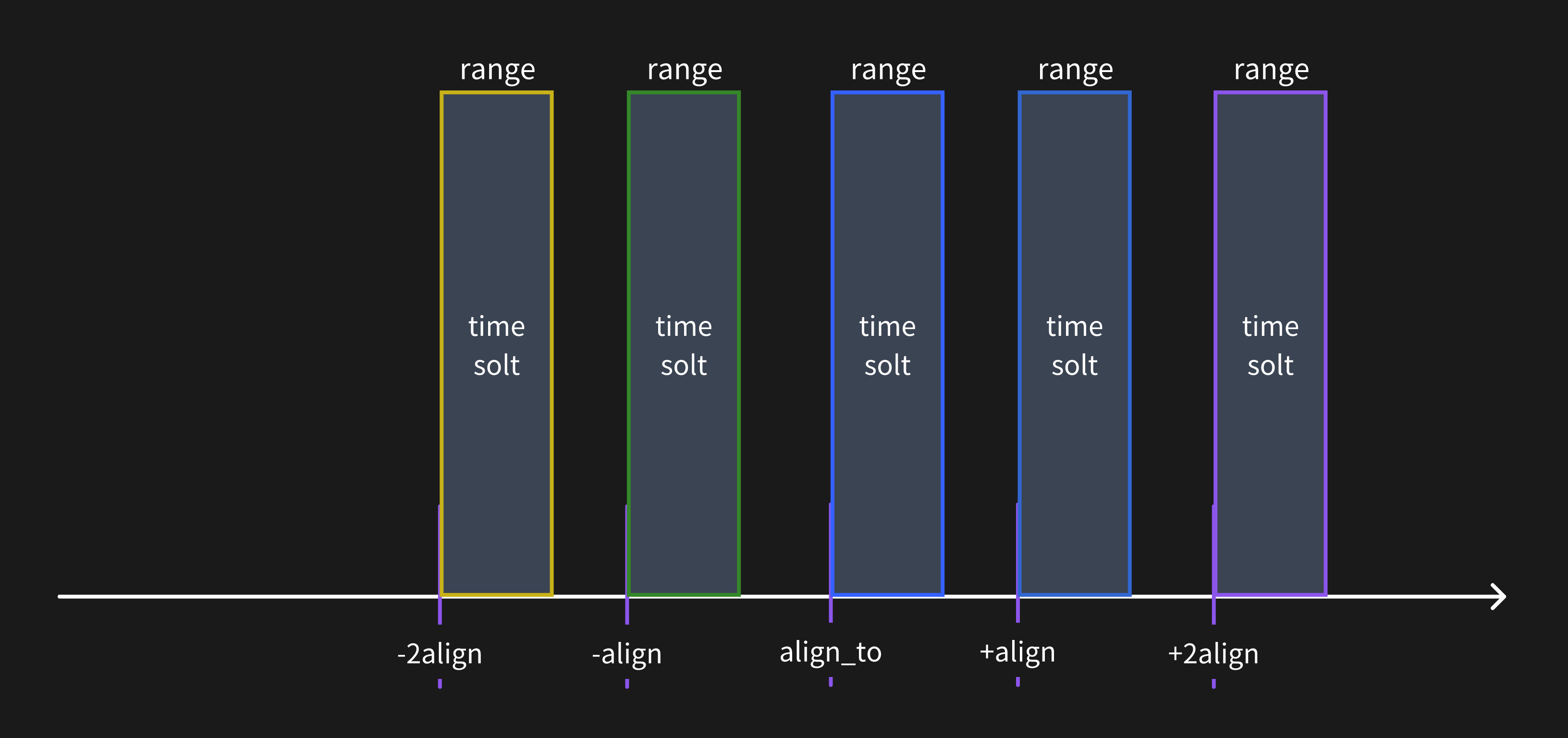
When the query resolution is less than the time range window, the metrics data will be calculated for multiple time range windows.
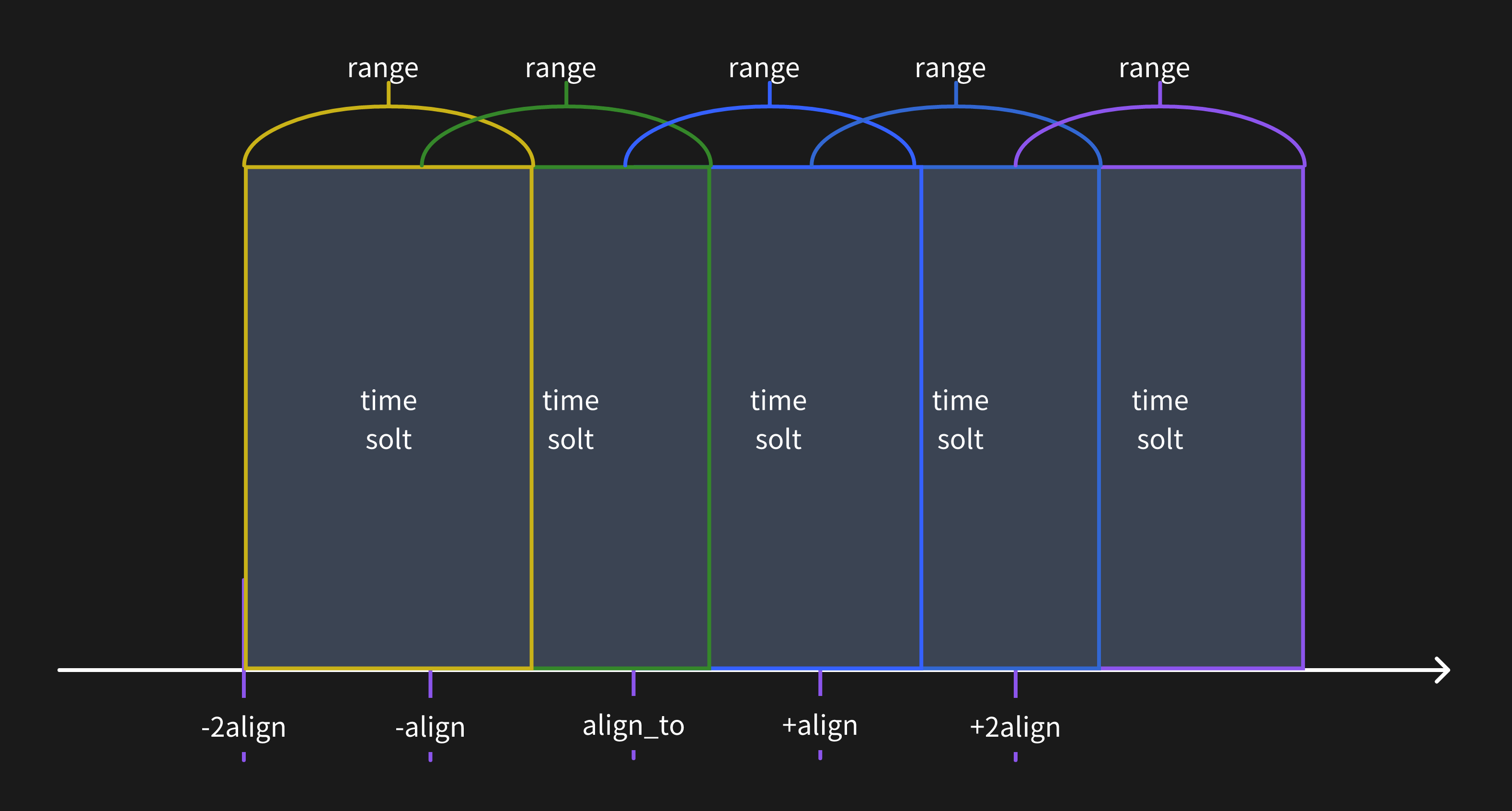
### Align to specific timestamp
The alignment times default based on the time zone of the current SQL client session.
You can change the origin alignment time to any timestamp you want. For example, use `NOW` to align to the current time:
```sql
SELECT
ts,
host,
avg(cpu) RANGE '1w'
FROM monitor
ALIGN '1d' TO NOW BY (host);
```
Or use a `ISO 8601` timestamp to align to a specified time:
```sql
SELECT
ts,
host,
avg(cpu) RANGE '1w'
FROM monitor
ALIGN '1d' TO '2023-12-01T00:00:00+08:00' BY (host);
```
### Fill null values
The `FILL` option can be used to fill null values in the data.
In the above example, the `LINEAR` method is used to fill null values.
Other methods are also supported, such as `PREV` and a constant value `X`.
For more information, please refer to the [FILL OPTION](/reference/sql/range.md#fill-option).
### Syntax
Please refer to [Range Query](/reference/sql/range.md) for more information.
## Table name constraints
If your table name contains special characters or uppercase letters,
you must enclose the table name in backquotes.
For examples, please refer to the [Table name constraints](/user-guide/deployments-administration/manage-data/basic-table-operations.md#table-name-constraints) section in the table creation documentation.
## HTTP API
Use POST method to query data:
```shell
curl -X POST \
-H 'authorization: Basic {{authorization if exists}}' \
-H 'Content-Type: application/x-www-form-urlencoded' \
-d 'sql=select * from monitor' \
http://localhost:4000/v1/sql?db=public
```
The result is shown below:
```json
{
"code": 0,
"output": [
{
"records": {
"schema": {
"column_schemas": [
{
"name": "host",
"data_type": "String"
},
{
"name": "ts",
"data_type": "TimestampMillisecond"
},
{
"name": "cpu",
"data_type": "Float64"
},
{
"name": "memory",
"data_type": "Float64"
}
]
},
"rows": [
["127.0.0.1", 1667446797450, 0.1, 0.4],
["127.0.0.1", 1667446798450, 0.5, 0.2],
["127.0.0.2", 1667446798450, 0.2, 0.3]
]
}
}
],
"execution_time_ms": 0
}
```
For more information about SQL HTTP request, please refer to [API document](/user-guide/protocols/http.md#post-sql-statements).
---
## View
In SQL, a view is a virtual table based on the result set of an SQL statement.
It contains rows and columns just like a real table.
The query of a view is run every time the view is referenced in a query.
In the following situations, you can use views:
* Simplifying complex queries, avoiding the need to repeatedly write and send complex statements for every query.
* Granting read permissions to specific users while restricting access to certain columns and rows to ensure data security and isolation.
A view is created with the `CREATE VIEW` statement.
## View examples
```sql
CREATE VIEW cpu_monitor AS
SELECT cpu, host, ts FROM monitor;
```
The view name is `cpu_monitor`, and the query statement after `AS` is the SQL statement to present the data. Query the view:
```sql
SELECT * FROM cpu_monitor;
```
```sql
+------+-----------+---------------------+
| cpu | host | ts |
+------+-----------+---------------------+
| 0.5 | 127.0.0.1 | 2023-12-13 02:05:41 |
| 0.3 | 127.0.0.1 | 2023-12-13 02:05:46 |
| 0.4 | 127.0.0.1 | 2023-12-13 02:05:51 |
| 0.3 | 127.0.0.2 | 2023-12-13 02:05:41 |
| 0.2 | 127.0.0.2 | 2023-12-13 02:05:46 |
| 0.2 | 127.0.0.2 | 2023-12-13 02:05:51 |
+------+-----------+---------------------+
```
Query view by `WHERE`:
```sql
SELECT * FROM cpu_monitor WHERE host = '127.0.0.2';
```
```sql
+------+-----------+---------------------+
| cpu | host | ts |
+------+-----------+---------------------+
| 0.3 | 127.0.0.2 | 2023-12-13 02:05:41 |
| 0.2 | 127.0.0.2 | 2023-12-13 02:05:46 |
| 0.2 | 127.0.0.2 | 2023-12-13 02:05:51 |
+------+-----------+---------------------+
```
Create a view that queries data from two tables:
```sql
CREATE VIEW app_cpu_monitor AS
SELECT cpu, latency, host, ts FROM monitor LEFT JOIN app_monitor
ON monitor.host = app_monitor.host AND monitor.ts = app_monitor.ts
```
Then query the view as if the data were coming from one single table:
```sql
SELECT * FROM app_cpu_monitor WHERE host = 'host1'
```
## Update View
`CREATE OR REPLACE VIEW` to update a view, if it doesn't exist, it will be created:
```sql
CREATE OR REPLACE VIEW memory_monitor AS
SELECT memory, host, ts FROM monitor;
```
## Shows the view definition
Shows the `CREATE VIEW` statement that creates the named view by `SHOW CREATE VIEW view_name`:
```sql
SHOW CREATE VIEW cpu_monitor;
```
```sql
+-------------+--------------------------------------------------------------+
| View | Create View |
+-------------+--------------------------------------------------------------+
| cpu_monitor | CREATE VIEW cpu_monitor AS SELECT cpu, host, ts FROM monitor |
+-------------+--------------------------------------------------------------+
```
## List Views
`SHOW VIEWS` statement to find all the views:
```sql
> SHOW VIEWS;
+----------------+
| Views |
+----------------+
| cpu_monitor |
| memory_monitor |
+----------------+
```
of course, just like `SHOW TABLES`, it supports `LIKE` and `WHERE`:
```sql
> SHOW VIEWS like 'cpu%';
+-------------+
| Views |
+-------------+
| cpu_monitor |
+-------------+
1 row in set (0.02 sec)
> SHOW VIEWS WHERE Views = 'memory_monitor';
+----------------+
| Views |
+----------------+
| memory_monitor |
+----------------+
```
## Drop View
Use `DROP VIEW` statement to drop a view:
```sql
DROP VIEW cpu_monitor;
```
To be quiet if it does not exist:
```sql
DROP VIEW IF EXISTS test;
```
---
## Time Zone
You can specify the time zone in the client session to manage time data conveniently.
The specified time zone in the client session does not affect the time data stored in the GreptimeDB server,
it only applies when the client sends a request to the server.
GreptimeDB converts the time value from a string representation to a datetime according to the specified time zone during ingestion or querying, or converts it back.
## Specify time zone in clients
By default, all clients use [the default time zone configuration](/user-guide/deployments-administration/configuration.md#default-time-zone-configuration), which is UTC.
You can also specify a time zone in each client session,
which will override the default time zone configuration.
### MySQL client
- **Command Line**: For configuring the time zone via the MySQL command line client, please refer to the [time zone section](/user-guide/protocols/mysql.md#time-zone) in the MySQL protocol documentation.
- **MySQL Driver**: If you are using MySQL Driver in Java or Go, see the [time zone section](/reference/sql-tools.md#time-zone) of the SQL tools documentation.
### PostgreSQL client
To configure the time zone for the PostgreSQL client, please refer to the [time zone section](/user-guide/protocols/postgresql.md#time-zone) in the PostgreSQL protocol documentation.
### HTTP API
When using the HTTP API, you can specify the time zone through the header parameter. For more information, please refer to the [HTTP API documentation](/user-guide/protocols/http.md#time-zone).
### Dashboard
The dashboard will use the local timezone as the default timezone value. You can change it in the settings menu.
### Other clients
For other clients, you can change [the default time zone configuration](/user-guide/deployments-administration/configuration.md#default-time-zone-configuration) of GreptimeDB.
## Impact of time zone on SQL statements
The client's time zone setting influences both data ingestion and querying.
### Ingest data
The time zone set in the client impacts the data during ingestion.
For more information, please refer to the [ingest data section](/user-guide/ingest-data/for-iot/sql.md#time-zone).
Additionally, the default timestamp values in the table schema are influenced by the client's time zone in the same manner as the ingested data.
### Query data
The time zone setting also affects data during querying.
For detailed information, please refer to the [query data section](/user-guide/query-data/sql.md#time-zone).
---
## Trace Data Modeling
:::warning
This section currently in the experimental stage and may be adjusted in future versions.
:::
In this section, we will cover how trace data is modeled in GreptimeDB as
tables.
We reuse the concept of Pipeline for trace data modeling. However, note that at
the moment, only built-in pipelines are supported.
## Data Model Versioning
First, the data types and features in GreptimeDB are evolving. For
forward-compatibility, we use the pipeline name for data model
versioning. Currently we have following pipeline for trace:
- `greptime_trace_v1`
It is required for user to specify this on OpenTelemetry OTLP/HTTP headers via
`x-greptime-pipeline-name: greptime_trace_v1`.
We may introduce new data model by adding new available pipeline names. And we
will keep previous pipeline supported. Note that new pipeline may not be
compatible with previous ones so you are recommended to use it in new table.
## Data Model
The `greptime_trace_v1` data model is pretty straight-forward. By default,
trace data is stored in a table named `opentelemetry_traces`. You can customize
the table name by specifying the `x-greptime-trace-table-name` header in your
OTLP/HTTP requests.
- It maps most common data fields from [OpenTelemetry
Trace](https://opentelemetry.io/docs/concepts/signals/traces/) data model to
GreptimeDB's table columns.
- `service_name` is extracted from `resource_attributes["service.name"]` and
used as a **Tag** (part of the **Primary Key**).
- `timestamp` is the start time of the span and is used as the **Time Index**.
- A new `duration_nano` column is generated using `end_time - start_time`.
- All attributes fields are flattened into columns using the name pattern:
`[span|resource|scope]_attributes.[attribute_key]`.
- Note: `resource_attributes.service.name` is excluded from flattening as it
is already stored in the `service_name` column.
- If the attribute value is a compound type like `Array` or `Kvlist`, it is
serialized to `JSON` type of GreptimeDB.
- Compound fields, `span_links` and `span_events` are stored as `JSON` type.
The table will be automatically generated when your first data item arrived. It
also follows our schema-less principle to update the table schema automatically
for new columns, for example, the new attribute fields.
A typical table structure generated from OpenTelemetry django instrument is like:
```
timestamp | 2025-05-07 10:03:29.657544
timestamp_end | 2025-05-07 10:03:29.661714
duration_nano | 4169970
trace_id | fb60d19aa36fdcb7d14a71ca0b9b42ae
span_id | 49806a2671f2ddcb
span_kind | SPAN_KIND_SERVER
span_name | POST todos/
span_status_code | STATUS_CODE_UNSET
span_status_message |
trace_state |
scope_name | opentelemetry.instrumentation.django
scope_version | 0.51b0
service_name | myproject
span_attributes.http.request.method | POST
span_attributes.url.full |
span_attributes.server.address | django:8000
span_attributes.network.peer.address |
span_attributes.server.port | 8000
span_attributes.network.peer.port |
span_attributes.http.response.status_code | 201
span_attributes.network.protocol.version | 1.1
resource_attributes.telemetry.sdk.language | python
resource_attributes.telemetry.sdk.name | opentelemetry
resource_attributes.telemetry.sdk.version | 1.30.0
span_events | []
span_links | []
parent_span_id | eccc18b6fc210f31
span_attributes.db.system |
span_attributes.db.name |
span_attributes.db.statement |
span_attributes.url.scheme | http
span_attributes.url.path | /todos/
span_attributes.client.address | 10.89.0.5
span_attributes.client.port | 44302
span_attributes.user_agent.original | python-requests/2.32.3
span_attributes.http.route | todos/
```
To check the table definition, you can use `show create table opentelemetry_traces`
statement. An output like this is expected:
```
Table | opentelemetry_traces
Create Table | CREATE TABLE IF NOT EXISTS "opentelemetry_traces" ( +
| "timestamp" TIMESTAMP(9) NOT NULL, +
| "timestamp_end" TIMESTAMP(9) NULL, +
| "duration_nano" BIGINT UNSIGNED NULL, +
| "trace_id" STRING NULL SKIPPING INDEX WITH(granularity = '10240', type = 'BLOOM'), +
| "span_id" STRING NULL, +
| "span_kind" STRING NULL, +
| "span_name" STRING NULL, +
| "span_status_code" STRING NULL, +
| "span_status_message" STRING NULL, +
| "trace_state" STRING NULL, +
| "scope_name" STRING NULL, +
| "scope_version" STRING NULL, +
| "service_name" STRING NULL SKIPPING INDEX WITH(granularity = '10240', type = 'BLOOM'),+
| "span_attributes.http.request.method" STRING NULL, +
| "span_attributes.url.full" STRING NULL, +
| "span_attributes.server.address" STRING NULL, +
| "span_attributes.network.peer.address" STRING NULL, +
| "span_attributes.server.port" BIGINT NULL, +
| "span_attributes.network.peer.port" BIGINT NULL, +
| "span_attributes.http.response.status_code" BIGINT NULL, +
| "span_attributes.network.protocol.version" STRING NULL, +
| "resource_attributes.telemetry.sdk.language" STRING NULL, +
| "resource_attributes.telemetry.sdk.name" STRING NULL, +
| "resource_attributes.telemetry.sdk.version" STRING NULL, +
| "span_events" JSON NULL, +
| "span_links" JSON NULL, +
| "parent_span_id" STRING NULL, +
| "span_attributes.db.system" STRING NULL, +
| "span_attributes.db.name" STRING NULL, +
| "span_attributes.db.statement" STRING NULL, +
| "span_attributes.url.scheme" STRING NULL, +
| "span_attributes.url.path" STRING NULL, +
| "span_attributes.client.address" STRING NULL, +
| "span_attributes.client.port" BIGINT NULL, +
| "span_attributes.user_agent.original" STRING NULL, +
| "span_attributes.http.route" STRING NULL, +
| TIME INDEX ("timestamp"), +
| PRIMARY KEY ("service_name") +
| ) +
| PARTITION ON COLUMNS ("trace_id") ( +
| trace_id < '1', +
| trace_id >= 'f', +
| trace_id >= '1' AND trace_id < '2', +
| trace_id >= '2' AND trace_id < '3', +
| trace_id >= '3' AND trace_id < '4', +
| trace_id >= '4' AND trace_id < '5', +
| trace_id >= '5' AND trace_id < '6', +
| trace_id >= '6' AND trace_id < '7', +
| trace_id >= '7' AND trace_id < '8', +
| trace_id >= '8' AND trace_id < '9', +
| trace_id >= '9' AND trace_id < 'a', +
| trace_id >= 'a' AND trace_id < 'b', +
| trace_id >= 'b' AND trace_id < 'c', +
| trace_id >= 'c' AND trace_id < 'd', +
| trace_id >= 'd' AND trace_id < 'e', +
| trace_id >= 'e' AND trace_id < 'f' +
| ) +
| ENGINE=mito +
| WITH( +
| append_mode = 'true', +
| table_data_model = 'greptime_trace_v1' +
| )
```
### Partition Rules
We included default [partition
rules](/user-guide/deployments-administration/manage-data/table-sharding.md#partition) for
trace table on the `trace_id` column based on the first character of it. This is
optimised for retrieve trace spans by the trace id.
The partition rule introduces 16 partitions for the table. It is suitable for a
3-5 datanode setup.
To customize the partition rule, you can create a new table ahead-of-time by
copying the DDL output by `show create table` on original table, update the
`PARTITION ON` section to include your own rules.
### Index
We include [skipping
index](/user-guide/manage-data/data-index.md#skipping-index) on `service_name`
and `trace_id` for most typical queries.
In real-world, you may want to speed up queries on other fields like an attribute
field. It's possible by apply additional index on these fields using [alter
table](/reference/sql/alter.md#create-an-index-for-a-column) statement.
Unlike partition rules, index can be created on existing table and be affective
on new data.
### Append-only Mode
By default, trace table created by OpenTelemetry API are in [append only
mode](/user-guide/deployments-administration/performance-tuning/design-table.md#when-to-use-append-only-tables).
### TTL
You can apply [TTL on trace table](/reference/sql/alter.md#alter-table-options).
## Auxiliary Tables
When you ingest trace data, GreptimeDB automatically creates two auxiliary
tables to facilitate searching for services and operations. These tables are
named by appending `_services` and `_operations` to your main trace table name.
By default, these are named `opentelemetry_traces_services` and
`opentelemetry_traces_operations`. If you customize the main trace table name
using the `x-greptime-trace-table-name` HTTP header, the auxiliary tables will
be named accordingly (e.g., `_services` and
`_operations`).
### Services Table (`opentelemetry_traces_services`)
This table stores the list of unique service names found in the trace data.
- **Columns**:
- `timestamp`: A constant timestamp (2100-01-01 00:00:00) used for all entries.
- `service_name`: The name of the service (Tag).
### Operations Table (`opentelemetry_traces_operations`)
This table stores the list of unique operations (service, span name, and span
kind) found in the trace data.
- **Columns**:
- `timestamp`: A constant timestamp (2100-01-01 00:00:00) used for all entries.
- `service_name`: The name of the service (Tag).
- `span_name`: The name of the span (Tag).
- `span_kind`: The kind of the span (Tag).
---
## Extending Trace Data
:::warning
This section currently in the experimental stage and may be adjusted in future versions.
:::
You can also generate derived data from trace. In this chapter, we will show you
some examples.
## Generate Aggregated Metrics from Trace
The span contains `duration_nano` field for span processing time. In this
example, we will create [Flow](/user-guide/flow-computation/overview.md) task to
generate latency metrics from trace data.
We will use OpenTelemetry Django instruments for source data. But the source
data doesn't really matter because fields used in this example are all generic
ones.
### Create Sink Table
First, we create a sink table which is a materialzed view in Flow. For latency
quantiles, we will use [uddsketch](https://arxiv.org/abs/2004.08604) for a quick
estimation of latency at given percentile.
```sql
CREATE TABLE "django_http_request_latency" (
"span_name" STRING NULL,
"latency_sketch" BINARY,
"time_window" TIMESTAMP time index,
PRIMARY KEY ("span_name")
);
```
This table contains 3 key columns:
- `span_name`: the type or name of span
- `latency_sketch`: the uddsketch data structure
- `time_window`: indicate the time window of current record
### Create Flow
Next we create a flow task to generate uddsketch data for every 30s time
window. The example filters spans by the scope name, which is optional depends
on your data.
Note: In this example, we use the default table name `opentelemetry_traces` as the source trace table. You should replace it with your own trace table name if it's customized.
```sql
CREATE FLOW django_http_request_latency_flow
SINK TO django_http_request_latency
EXPIRE AFTER '30m'
COMMENT 'Aggregate latency using uddsketch'
AS
SELECT
span_name,
uddsketch_state(128, 0.01, "duration_nano") AS "latency_sketch",
date_bin('30 seconds'::INTERVAL, "timestamp") as "time_window",
FROM opentelemetry_traces
WHERE
scope_name = 'opentelemetry.instrumentation.django'
GROUP BY
span_name,
time_window;
```
### Query Metrics
The sink table will be filled with aggregated data as trace data ingested. We
can use following SQL to get p90 latency of the each span.
```sql
SELECT
span_name,
time_window,
uddsketch_calc(0.90, "latency_sketch") AS p90
FROM
django_http_request_latency
ORDER BY
time_window DESC
LIMIT 20;
```
The query will return results like:
```
span_name | time_window | p90
---------------------+----------------------------+--------------------
GET todos/ | 2025-05-09 02:38:00.000000 | 4034758.586053441
POST todos/ | 2025-05-09 02:38:00.000000 | 22988738.680499777
PUT todos// | 2025-05-09 02:38:00.000000 | 5338559.200101535
GET todos/ | 2025-05-09 02:37:30.000000 | 4199425.807196321
POST todos/ | 2025-05-09 02:37:30.000000 | 15104466.164886404
PUT todos// | 2025-05-09 02:37:30.000000 | 16693072.385310777
GET todos/ | 2025-05-09 02:37:00.000000 | 4370813.453648573
POST todos/ | 2025-05-09 02:37:00.000000 | 30417369.407361753
PUT todos// | 2025-05-09 02:37:00.000000 | 14512192.224492861
GET todos/ | 2025-05-09 02:36:30.000000 | 3578495.53232116
POST todos/ | 2025-05-09 02:36:30.000000 | 15409606.895490168
PUT todos// | 2025-05-09 02:36:30.000000 | 15409606.895490168
GET todos/ | 2025-05-09 02:36:00.000000 | 3507634.2346514342
POST todos/ | 2025-05-09 02:36:00.000000 | 45377987.991290994
PUT todos// | 2025-05-09 02:36:00.000000 | 14512192.224492861
GET todos/ | 2025-05-09 02:35:30.000000 | 3237945.86410019
POST todos/ | 2025-05-09 02:35:30.000000 | 15409606.895490168
PUT todos// | 2025-05-09 02:35:30.000000 | 13131130.769316385
GET todos/ | 2025-05-09 02:35:00.000000 | 3173828.124217018
POST todos/ | 2025-05-09 02:35:00.000000 | 14512192.224492861
(20 rows)
```
---
## Traces
:::warning
This section currently in the experimental stage and may be adjusted in future versions.
:::
Native support for Trace data is introduced since GreptimeDB v0.14. In this
section we will cover from basic ingestion and query steps, to advanced
internals of data modeling.
- [Ingestion and Query](./read-write.md)
- [Trace Data Modeling in GreptimeDB](./data-model.md)
- [Extending Trace Data](./extend-trace.md)
---
## Ingestion and Query
:::warning
This section currently in the experimental stage and may be adjusted in future versions.
:::
In this section, we will get started with trace data in GreptimeDB from
ingestion and query.
GreptimeDB doesn't invent new protocols for trace, it follows existing standard
and widely adopted protocols.
## Ingestion
GreptimeDB uses OpenTelemetry OTLP/HTTP protocol as the primary trace data
ingestion protocol. OpenTelemetry Trace is the most adopted subprotocol in
OpenTelemetry family.
### OpenTelemetry SDK
If OpenTelemetry SDK/API is used in your application, you can configure an
OTLP/HTTP exporter to write trace data directly to GreptimeDB.
We covered this part in our [OpenTelemetry protocol
docs](/user-guide/ingest-data/for-observability/opentelemetry.md). You can
follow the guide for endpoint and parameters.
### OpenTelemetry Collector
[OpenTelemetry Collector](https://opentelemetry.io/docs/collector/) is a
vendor-neutral service for collecting and processing OpenTelemetry data. You can
also configure it to send trace data to GreptimeDB using OTLP/HTTP.
#### Start OpenTelemetry Collector
You can use the following command to quickly start an OpenTelemetry Collector
instance, which will listen on ports `4317` (gRPC) and `4318` (HTTP):
```shell
docker run --rm \
--network host \
-p 4317:4317 \
-p 4318:4318 \
-v $(pwd)/config.yaml:/etc/otelcol-contrib/config.yaml \
otel/opentelemetry-collector-contrib:0.123.0
```
The content of the `config.yaml` file is as follows:
```yaml
receivers:
otlp:
protocols:
grpc:
endpoint: 0.0.0.0:4317
http:
endpoint: 0.0.0.0:4318
exporters:
otlphttp:
endpoint: "http://greptimedb:4000/v1/otlp" # Replace greptimedb with your setup
headers:
x-greptime-pipeline-name: "greptime_trace_v1"
#authorization: "Basic "
tls:
insecure: true
service:
pipelines:
traces:
receivers: [otlp]
exporters: [otlphttp]
```
#### Write Trace Data to OpenTelemetry Collector
You can configure the corresponding exporter to write traces data to the
OpenTelemetry Collector. For example, you can use the environment variable
`OTEL_EXPORTER_OTLP_TRACES_ENDPOINT` to configure the endpoint of the exporter:
```shell
export OTEL_EXPORTER_OTLP_TRACES_ENDPOINT="http://localhost:4318/v1/otlp/v1/traces"
```
For convenience, you can use the tool
[`telemetrygen`](https://github.com/open-telemetry/opentelemetry-collector-contrib/tree/main/cmd/telemetrygen)
to quickly generate traces data and write it to the OpenTelemetry Collector. For
more details, please refer to the [OpenTelemetry Collector official
documentation](https://opentelemetry.io/docs/collector/quick-start/).
You can use the following command to install `telemetrygen` (please ensure you
have installed Go):
```shell
go install github.com/open-telemetry/opentelemetry-collector-contrib/cmd/telemetrygen@latest
```
Then you can use the following command to generate traces data and write it to
the OpenTelemetry Collector:
```shell
telemetrygen traces --otlp-insecure --traces 3
```
The above command will generate 3 traces data and write it to the OpenTelemetry
Collector via gRPC protocol, and eventually stored into GreptimeDB.
### Authorization
The GreptimeDB OTEL endpoint supports Basic authentication. For details, please refer to the [authentication](/user-guide/protocols/http.md#authentication) documentation.
### GreptimeDB Pipeline
The HTTP header `x-greptime-pipeline-name` is required for ingesting trace
data. Here we reuse the Pipeline concept of GreptimeDB for data
transformation. However, note that we only support built-in `greptime_trace_v1`
as the pipeline for tracing. No custom pipeline is allowed for the moment.
### Append-only Mode
By default, trace table created by OpenTelemetry API are in [append only
mode](/user-guide/deployments-administration/performance-tuning/design-table.md#when-to-use-append-only-tables).
## Query
To query the trace data, GreptimeDB has two types of API provided. The Jaeger
compatible API and GreptimeDB's original SQL based query interfaces, which is
available in HTTP, MySQL and Postgres protocols.
### Jaeger
We build Jaeger compatibility layer into GreptimeDB so you can reuse your Jaeger
frontend or any other integrations like Grafana's Jaeger data source.
For detail of Jaeger's endpoint and parameters, check [our Jaeger protocol
docs](/user-guide/query-data/jaeger.md).
### SQL
All data in GreptimeDB is available for query using SQL, via MySQL and other
transport protocol.
By default, trace data is written into the table called
`opentelemetry_traces`. The table name is customizable via header
`x-greptime-trace-table-name`. You can run SQL queries against the table:
```sql
SELECT * FROM public.opentelemetry_traces \G
```
An example output is like
```
*************************** 1. row ***************************
timestamp: 2025-05-07 10:03:29.657544
timestamp_end: 2025-05-07 10:03:29.661714
duration_nano: 4169970
parent_span_id: eccc18b6fc210f31
trace_id: fb60d19aa36fdcb7d14a71ca0b9b42ae
span_id: 49806a2671f2ddcb
span_kind: SPAN_KIND_SERVER
span_name: POST todos/
span_status_code: STATUS_CODE_UNSET
span_status_message:
trace_state:
scope_name: opentelemetry.instrumentation.django
scope_version: 0.51b0
service_name: myproject
span_attributes.http.request.method: POST
span_attributes.url.full:
span_events: []
span_links: []
...
```
We will cover more information about the table structure in [Data
Model](./data-model.md) section.
---
## Vector Data Type
## Overview
In the field of artificial intelligence, vectors are an important data type used to represent features or samples within a dataset. Vectors are utilized in various machine learning and deep learning algorithms, such as recommendation systems, natural language processing, and image recognition. By introducing the vector type, GreptimeDB enables more efficient support for these AI applications, offering robust vector storage and computation capabilities.
## Basic Introduction to Vector Type
In GreptimeDB, a vector is represented as an array of Float32 (32-bit floating-point) with a fixed dimension. When creating a vector type column, the dimension must be specified and cannot be changed afterward.
## Defining a Vector Type Column
In SQL, a table with a vector type column can be defined using the following syntax. Note that the dimension `