Design Your Table Schema

The design of your table schema significantly impacts both write and query performance. Before writing data, it is crucial to understand the data types, scale, and common queries relevant to your business, then model the data accordingly.

Designing a table comes down to a few decisions:

• which columns form the primary key (data ordering and time-series identity);
• whether the table is append-only or deduplicates, and which merge mode to use;
• which columns to index;
• how to lay out your data across tables (one wide table vs. multiple tables) and how to partition them for scale.

This guide first explains how GreptimeDB stores and reads data, then walks through each of these decisions in turn.

Basic Concepts

Before proceeding, please review the GreptimeDB Data Model Documentation.

Cardinality

Cardinality: Refers to the number of unique values in a dataset. It can be classified as "high cardinality" or "low cardinality":

• Low Cardinality: Low cardinality columns usually have constant values. The total number of unique values usually no more than 10 thousand. For example, namespace, cluster, http_method are usually low cardinality.
• High Cardinality: High cardinality columns contain a large number of unique values. For example, trace_id, span_id, user_id, uri, ip, uuid, request_id, table auto increment id, timestamps are usually high cardinality.

Semantic Types

In GreptimeDB, columns are categorized into three semantic types: Tag, Field, and Timestamp. The timestamp usually represents the time of data sampling or the occurrence time of logs/events. GreptimeDB uses the TIME INDEX constraint to identify the Timestamp column. So the Timestamp column is also called the TIME INDEX column. If you have multiple columns with timestamp data type, you can only define one as TIME INDEX and others as Field columns.

In GreptimeDB, tag columns are optional. GreptimeDB reuses the PRIMARY KEY constraint to define tag columns; together they identify a time series and define how rows are ordered in storage (see How GreptimeDB Stores and Reads Data). The main purposes of tag columns are:

1. Defining the storage ordering of data, which improves the locality of data with the same tags. If there are no tag columns, GreptimeDB sorts rows by timestamp.
2. Identifying a unique time series, so GreptimeDB can deduplicate rows under the same time series (primary key) when the table is not append-only.
3. Smoothing migration from other TSDBs that use tags or labels.

How GreptimeDB Stores and Reads Data

Understanding how GreptimeDB stores data and executes a query makes the rest of this guide easier to follow. Later sections refer back to the ideas introduced here. For the engine-level details — the on-disk SST file format and the full pruning pipeline — see Data Layout in SST Files and Scan Pruning in the storage engine documentation.

Data is sorted by primary key and time

GreptimeDB stores rows sorted by (primary key, timestamp). Rows that share the same primary key form a single time series and are stored next to each other, ordered by time. This locality is what makes scanning a single time series cheap and improves compression. For a concrete example of how rows are laid out on disk, see Data Layout in SST Files.

A scan prunes data in stages

GreptimeDB stores data in immutable files (SST files). Each file is split into row groups, and each row group keeps statistics such as the minimum and maximum value of every column. When you run a query, GreptimeDB avoids reading data that cannot match, in increasingly precise stages:

1. Time range: skip whole files (and in-memory buffers) whose time range does not overlap the query's time range. This is usually the cheapest and most effective step for time-series data.
2. Row-group min/max statistics: within a file, skip row groups whose statistics prove that no row can match a filter.
3. Index: if a filtered column has an index, use it to further narrow down to specific row groups or rows.
4. Read and filter: read the remaining data and apply the exact filters.

Take a query over a host_metrics table with PRIMARY KEY (host, region) as an example:

SELECT ts, cpu
FROM host_metrics
WHERE host = 'host-a'
  AND region = 'us-east'
  AND ts >= '2024-01-01 10:00:00'
  AND ts < '2024-01-01 11:00:00'
  AND cpu > 0.7;

Time range removes any file whose data falls outside the one-hour window.

Primary-key ordering keeps all host-a / us-east rows together, so the scan reads a small contiguous slice of each remaining file instead of the whole file.

Row-group statistics on the first primary-key column are especially effective. Because rows are sorted by primary key, the leading primary-key column (host) has a tight, non-overlapping range in each row group:

Row group	host (min..max)
0	host-a .. host-b
1	host-c .. host-f

The filter host = 'host-a' can only match row group 0, so row group 1 is skipped without being read. Choosing and ordering the primary key well turns the leading primary-key column into an effective coarse pruning key — no extra index required. This pruning is coarse, though: GreptimeDB keeps no global index over the primary key, so it cannot jump straight to the rows for a given key. It only skips row groups by their min/max values, which works well for the leading primary-key column but does little for columns deeper in the key or for point lookups on high cardinality columns — that is what indexes are for. Statistics on field columns help too: a row group whose cpu maximum is 0.6 is skipped for cpu > 0.7.

Indexes handle selective filters that ordering and statistics cannot. For example, an index on a column lets the scan jump to the matching row groups or rows before decoding the data columns. See Index.

Deduplication happens during the scan

GreptimeDB uses an LSM-tree storage engine: it never overwrites data in place, so multiple versions of the same row can exist across files. For tables that are not append-only, the scan merges and deduplicates rows that share the same (primary key, timestamp) on the fly, keeping only the newest version (see Data updating and merging).

Append-only tables skip this work. They don't need to deduplicate, and when a query doesn't require ordered output they can be scanned in any order, which is faster.

Takeaways

• Filtering by time range and by the leading primary-key columns is the cheapest way to make queries fast.
• Indexes help selective filters on columns that ordering doesn't cover.
• Deduplication (on non-append-only tables) adds extra work at query time.

Primary key

The primary key is the most impactful schema decision: it defines how rows are ordered on disk and identifies a time series for deduplication. This section helps you decide whether to set one and which columns to use.

Primary key is optional

Bad primary key or index may significantly degrade performance. Generally you can create an append-only table without a primary key since ordering data by timestamp is sufficient for many workloads. It can also serve as a baseline.

CREATE TABLE http_logs (
  access_time TIMESTAMP TIME INDEX,
  application STRING,
  remote_addr STRING,
  http_status STRING,
  http_method STRING,
  http_refer STRING,
  user_agent STRING,
  request_id STRING,
  request STRING,
) with ('append_mode'='true');

The http_logs table is an example for storing HTTP server logs.

• The 'append_mode'='true' option creates the table as an append-only table. This ensures a log doesn't override another one with the same timestamp.
• The table sorts logs by time so it is efficient to search logs by time.

Primary key design

You can use primary key when there are suitable columns and one of the following conditions is met:

• Most queries can benefit from the ordering.
• You need to deduplicate (including delete) rows by the primary key and time index.

For example, if you always only query logs of a specific application, you may set the application column as primary key (tag).

SELECT message FROM http_logs WHERE application = 'greptimedb' AND access_time > now() - '5 minute'::INTERVAL;

The number of applications is usually limited. Table http_logs_v2 uses application as the primary key. It sorts logs by application so querying logs under the same application is faster as it only has to scan a small number of rows. Setting tags may also reduce disk space usage as it improves the locality of data.

CREATE TABLE http_logs_v2 (
  access_time TIMESTAMP TIME INDEX,
  application STRING,
  remote_addr STRING,
  http_status STRING,
  http_method STRING,
  http_refer STRING,
  user_agent STRING,
  request_id STRING,
  request STRING,
  PRIMARY KEY(application),
) with ('append_mode'='true');

A long primary key will negatively affect the insert performance and enlarge the memory footprint. It's recommended to define a primary key with no more than 5 columns.

You can put high cardinality columns such as trace_id, span_id, or user_id into the primary key, but it is often not the best way to filter on them.

Adding a high cardinality column to the primary key has a cost but limited benefit:

• It makes the primary key longer, which slows inserts and uses more memory.
• On deduplicating tables, deduplication by a high cardinality key is expensive. If you can tolerate duplication, use an append-only table instead.
• Unlike a skipping index, it doesn't always speed up queries much.

A skipping index targets the same filters with much lower overhead, so it is usually the better default. Add a high cardinality column to the primary key only when you genuinely need to order or deduplicate by it. Because the best layout depends on your data and queries, benchmark on your own dataset to decide.

Recommendations for tags:

• Low cardinality columns that occur in WHERE/GROUP BY/ORDER BY frequently. These columns usually remain constant. For example, namespace, cluster, or an AWS region.
• No need to set all low cardinality columns as tags since this may impact the performance of ingestion and querying.
• Typically use short strings and integers for tags, avoiding FLOAT, DOUBLE, TIMESTAMP.
• For high cardinality columns such as trace_id, span_id, and user_id, prefer a skipping index; add them to the primary key only when you need to order or deduplicate by them.
• Order primary key columns from the most frequently filtered and most selective leading column. The leading column benefits the most from ordering and row-group pruning (see How GreptimeDB Stores and Reads Data).

Deduplication and Append-Only

Next, decide how the table handles rows that share the same primary key and timestamp:

• Append-only (append_mode = 'true'): keep every row, with no deduplication or deletes. This is the fastest option.
• Deduplicating (the default): keep a single row per (primary key, timestamp), with a merge mode (last_row or last_non_null) controlling how updates combine.

Choose append-only when you don't need updates or deletes (for example, logs). Otherwise, use the default deduplicating mode, which keeps append_mode at false and removes duplicate rows by primary key and timestamp.

Because deduplication groups rows by (primary key, timestamp), the primary key decides what counts as a duplicate. Make sure the primary key uniquely identifies a time series, so that rows you want to keep separate are not merged together (see Primary key).

For example, the system_metrics table deduplicates rows by host and ts:

CREATE TABLE IF NOT EXISTS system_metrics (
  host STRING,
  cpu_util DOUBLE,
  memory_util DOUBLE,
  disk_util DOUBLE,
  ts TIMESTAMP DEFAULT CURRENT_TIMESTAMP,
  PRIMARY KEY(host),
  TIME INDEX(ts)
);

Data updating and merging

GreptimeDB supports two different strategies for deduplication: last_row and last_non_null. You can specify the strategy by the merge_mode table option.

merge_mode only takes effect on deduplicating tables. Append-only tables don't merge rows, so you normally leave merge_mode unset on them.

GreptimeDB uses an LSM Tree-based storage engine, which does not overwrite old data in place but allows multiple versions of data to coexist. These versions are merged during the query process. The default merge behavior is last_row, meaning the most recently inserted row takes precedence.

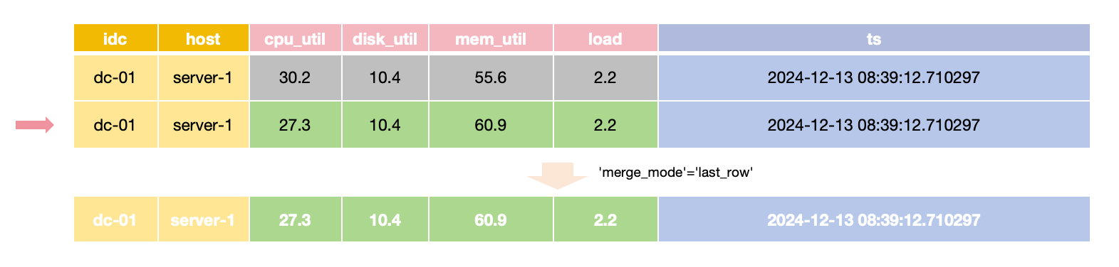
In last_row merge mode, the latest row is returned for queries with the same primary key and time value, requiring all Field values to be provided during updates.

For scenarios where only specific Field values need updating while others remain unchanged, the merge_mode option can be set to last_non_null. This mode retains the latest non-null value for each field during queries, allowing updates to provide only the values that need to change.

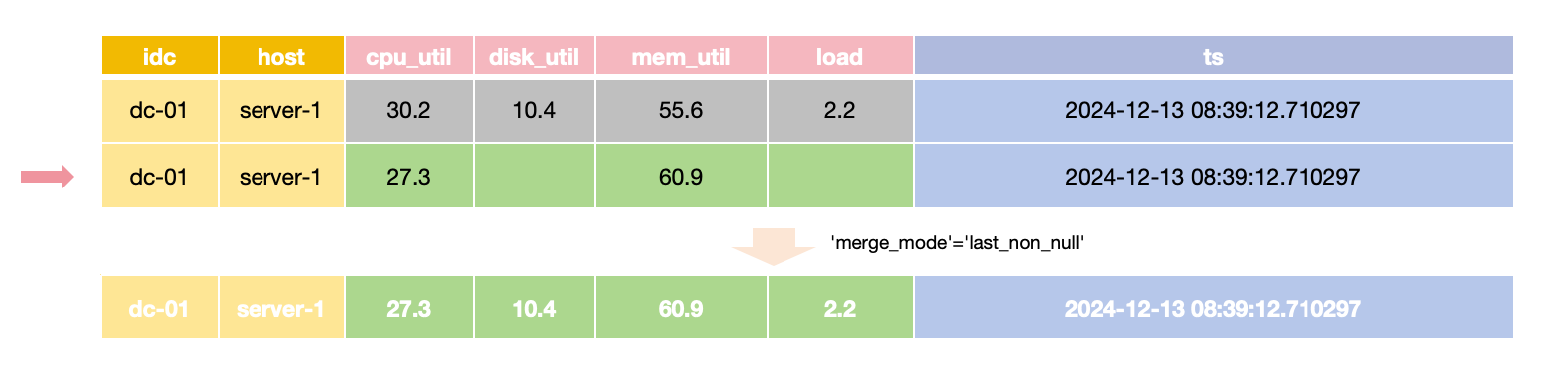
Tables auto-created via the InfluxDB line protocol default to last_non_null to align with InfluxDB's update behavior, configurable via the influxdb.default_merge_mode option.

The last_row merge mode doesn't have to check each individual field value so it is usually faster than the last_non_null mode.

Deduplication and partitioning

Deduplication and merging happen within a single partition. If you partition a deduplicating table (any table that is not append-only) by a column that is not part of the primary key, rows with the same primary key can be spread across different partitions and won't be deduplicated against each other.

To keep deduplication correct, only use primary key columns as partition columns, so that rows with the same primary key always go to the same partition. GreptimeDB does not enforce this — it is your responsibility. See Distributed Tables.

When to use append-only tables

If you don't need the following features, you can use append-only tables:

• Deduplication
• Deletion

GreptimeDB implements DELETE via deduplicating rows so append-only tables don't support deletion now. Deduplication requires more computation and restricts the parallelism of ingestion and querying. Using append-only tables usually has better query performance.

Index

With the primary key and table mode decided, you can add indexes to speed up specific filters. Indexes are optional — add one only when a filter is common and not already fast enough, and choose the index type based on the column (see the comparison in When to use index).

A primary key and an index are complementary, not alternatives:

• The primary key gives every table one physical ordering. It helps range scans and locality, and is required for deduplication and deletion.
• An index is auxiliary and can be added to any column, whether a tag or a field. It targets selective filters (for example a point lookup on a high cardinality column) that ordering alone can't accelerate.

A single query can use both at once. For example, with a primary key on application and a skipping index on request_id, GreptimeDB uses the time range and the application ordering to read a small slice of data, then uses the index on request_id to pinpoint the matching rows.

Inverted Index

GreptimeDB supports inverted index that may speed up filtering low cardinality columns. When creating a table, you can specify the inverted index columns using the INVERTED INDEX clause. For example, http_logs_v3 adds an inverted index for the http_method column.

CREATE TABLE http_logs_v3 (
  access_time TIMESTAMP TIME INDEX,
  application STRING,
  remote_addr STRING,
  http_status STRING,
  http_method STRING INVERTED INDEX,
  http_refer STRING,
  user_agent STRING,
  request_id STRING,
  request STRING,
  PRIMARY KEY(application),
) with ('append_mode'='true');

The following query can use the inverted index on the http_method column.

SELECT message FROM http_logs_v3 WHERE application = 'greptimedb' AND http_method = `GET` AND access_time > now() - '5 minute'::INTERVAL;

Inverted index supports the following operators:

• =
• <
• <=
• >
• >=
• IN
• BETWEEN
• ~

Skipping Index

For high cardinality columns like trace_id, request_id, a skipping index is often a good fit. This method has lower storage overhead and resource usage, particularly in terms of memory and disk consumption.

Example:

CREATE TABLE http_logs_v4 (
  access_time TIMESTAMP TIME INDEX,
  application STRING,
  remote_addr STRING,
  http_status STRING,
  http_method STRING INVERTED INDEX,
  http_refer STRING,
  user_agent STRING,
  request_id STRING SKIPPING INDEX,
  request STRING,
  PRIMARY KEY(application),
) with ('append_mode'='true');

The following query can use the skipping index to filter the request_id column.

SELECT message FROM http_logs_v4 WHERE application = 'greptimedb' AND request_id = `25b6f398-41cf-4965-aa19-e1c63a88a7a9` AND access_time > now() - '5 minute'::INTERVAL;

However, note that the query capabilities of the skipping index are generally inferior to those of the inverted index. Skipping index can't handle complex filter conditions and may have a lower filtering performance on low cardinality columns. It only supports the equal operator.

Full-Text Index

For unstructured log messages that require tokenization and searching by terms, GreptimeDB provides full-text index.

For example, the raw_logs table stores unstructured logs in the message field.

CREATE TABLE IF NOT EXISTS `raw_logs` (
  message STRING NULL FULLTEXT INDEX WITH(analyzer = 'English', case_sensitive = 'false'),
  ts TIMESTAMP(9) NOT NULL,
  TIME INDEX (ts),
) with ('append_mode'='true');

The message field is full-text indexed using the FULLTEXT INDEX option. See fulltext column options for more information.

Storing and querying structured logs usually have better performance than unstructured logs with full-text index. It's recommended to use Pipeline to convert logs into structured logs.

When to use index

Index in GreptimeDB is flexible and powerful. You can create an index for any column, no matter if the column is a tag or a field. It's meaningless to create additional index for the timestamp column. Generally you don't need to create indexes for all columns. Maintaining indexes may introduce additional cost and stall ingestion. A bad index may occupy too much disk space and make queries slower.

You can use a table without additional index as a baseline. There is no need to create an index for the table if the query performance is already acceptable. You can create an index for a column when:

• The column occurs in the filter frequently.
• Filtering the column without an index isn't fast enough.
• There is a suitable index for the column.

The following table lists the suitable scenarios of all index types.

	Inverted Index	Full-Text Index	Skip Index
Suitable Scenarios	- Filtering low cardinality columns	- Text content search	- Precise filtering high cardinality columns
Creation Method	- Specified using INVERTED INDEX	- Specified using FULLTEXT INDEX in column options	- Specified using SKIPPING INDEX in column options

Wide Table vs. Multiple Tables

With each table's schema settled, decide how to spread your data across tables: group columns collected together into one wide table, use separate tables for logically distinct data, and partition a table only when a single node can no longer serve it.

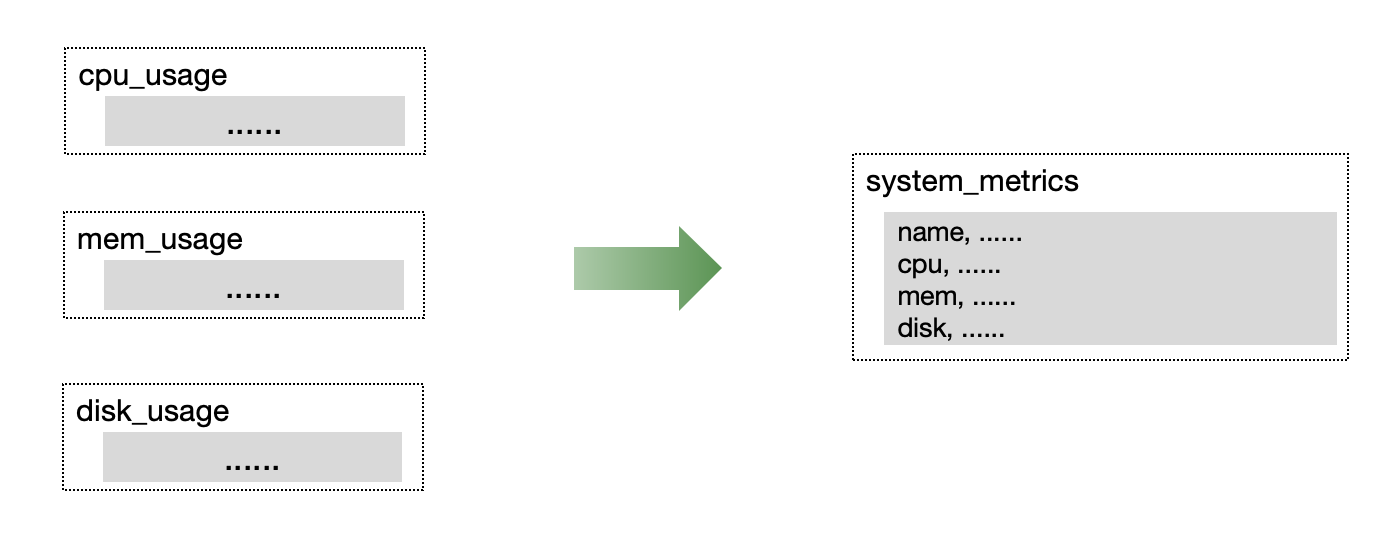
In monitoring or IoT scenarios, multiple metrics are often collected simultaneously. We recommend placing metrics collected simultaneously into a single table to improve read/write throughput and data compression efficiency.

Prometheus metrics and the metric engine

For Prometheus-style metrics, GreptimeDB relies on the Metric Engine. If you ingest data through the Prometheus remote write API, GreptimeDB routes it to the metric engine automatically: tables are created for you and no configuration is needed.

Under the hood, the metric engine handles Prometheus's single-value model efficiently by storing many small metric tables on a shared physical wide table. Each metric stays its own logical table, while the shared storage improves read/write throughput and compression.

When you scale out to a cluster, one detail matters: partitioning. By default, the metric engine uses a single physical table with only one partition, which is enough for most workloads. In a cluster, however, that means a single datanode handles all ingestion. To spread the load across nodes, create your own partitioned physical table on a suitable label such as namespace. See GreptimeDB cluster with metric engine for an example.

Multiple tables vs. multiple partitions

Splitting data into multiple tables and partitioning a single table solve different problems and can be combined:

• Use multiple tables when data is logically distinct: different schemas, different sets of columns, or different retention (TTL) requirements. Separate tables also let each table use its own primary key, indexes, and merge mode, whereas a single wide table has to share one of each across all its columns. They keep each schema clean and let you tune and retain each table independently. The cost is more tables: because each table maintains its own files, splitting data across many small tables produces many small files.
• Use multiple partitions (a distributed table) when a single table grows too large for one node to serve. Partitioning splits one table's rows across nodes for horizontal scaling while keeping the data in a single table, so it spreads load without creating as many small files as many separate tables would. See Distributed Tables.

In short: split into separate tables for logical separation, and into partitions for scale.

Distributed Tables

GreptimeDB supports partitioning data tables to distribute read/write hotspots and achieve horizontal scaling. This section continues from the layout discussion above and helps you decide whether to partition a table, how many partitions to create, and which columns to partition on.

Two misunderstandings about distributed tables

As a time-series database, GreptimeDB automatically partitions data based on the TIME INDEX column at the storage layer. Therefore, it is unnecessary and not recommended for you to partition data by time (e.g., one partition per day or one table per week).

Additionally, GreptimeDB is a columnar storage database, so partitioning a table refers to horizontal partitioning by rows, with each partition containing all columns.

When to Partition and Determining the Number of Partitions

A table can utilize all the resources in the machine, especially during query. Partitioning a table may not always improve the performance:

• A distributed query plan isn't always as efficient as a local query plan.
• Distributed query may introduce additional data transmission across the network.

There is no need to partition a table unless a single machine isn't enough to serve the table. For example:

• There is not enough local disk space to store the data or to cache the data when using object stores.
• You need more CPU cores to improve the query performance or more memory for costly queries.
• The disk throughput becomes the bottleneck.
• The ingestion rate is larger than the throughput of a single node.

GreptimeDB releases a benchmark report with each major version update, detailing the ingestion throughput of a single partition. Use this report alongside your target scenario to estimate if the write volume approaches the single partition's limit.

To estimate the total number of partitions, consider the write throughput and reserve an additional 50% resource of CPU to ensure query performance and stability. Adjust this ratio as necessary. You can reserve more CPU cores if there are more queries.

How to choose partition columns

GreptimeDB employs expressions to define partitioning rules. For optimal performance, select partition columns that are:

• Evenly distributed: each partition should receive a similar share of data, so no single partition becomes a hotspot. The column should have enough distinct values to divide the data.
• Stable: the value should not change for a given entity over time.
• Aligned with query conditions: the column should appear in the filters of your common queries, so a query can be routed to a small number of partitions instead of all of them.

Examples include:

• Partitioning by the prefix of a trace id.
• Partitioning by data center name.
• Partitioning by business name.

For instance, if most queries target data from a specific data center, using the data center name as a partition column is appropriate. If the data distribution is not well understood, perform aggregate queries on existing data to gather relevant information.

Partition columns and deduplication

If your table is not append-only (deduplication is enabled), the partition columns must be a subset of the primary key columns. Deduplication and merging only happen within a partition, so rows with the same primary key must always be routed to the same partition. Partitioning on a non-primary-key column would scatter rows with the same primary key across partitions and break deduplication. Append-only tables don't deduplicate, so they can be partitioned by any column. See Data updating and merging.

For more details, refer to the table partition guide.

SST format

This is an upgrade-only note; you don't normally need it when designing a new table.

GreptimeDB stores data in SST files using the flat format by default. It works well across all primary key cardinalities — including high cardinality ones such as trace_id or uuid — so you are not expected to set the sst_format option manually.

The only reason to set sst_format is when upgrading from an old version of GreptimeDB. Older versions used a legacy primary_key format as the default. If you upgraded from such a version, or are not sure which format a table currently uses, switch it to flat:

ALTER TABLE http_logs_v2 SET 'sst_format' = 'flat';

See SST formats for more details.