SQL
GreptimeDB supports full SQL for querying data from a database.
In this document, we will use the monitor table to demonstrate how to query data.
For instructions on creating the monitor table and inserting data into it,
Please refer to table management and Ingest Data.
Basic query
The query is represented by the SELECT statement.
For example, the following query selects all data from the monitor table:
SELECT * FROM monitor;
The query result looks like the following:
+-----------+---------------------+------+--------+
| host      | ts                  | cpu  | memory |
+-----------+---------------------+------+--------+
| 127.0.0.1 | 2022-11-03 03:39:57 |  0.1 |    0.4 |
| 127.0.0.1 | 2022-11-03 03:39:58 |  0.5 |    0.2 |
| 127.0.0.2 | 2022-11-03 03:39:58 |  0.2 |    0.3 |
+-----------+---------------------+------+--------+
3 rows in set (0.00 sec)
Functions are also supported in the SELECT field list.
For example, you can use the count() function to retrieve the total number of rows in the table:
SELECT count(*) FROM monitor;
+-----------------+
| COUNT(UInt8(1)) |
+-----------------+
|               3 |
+-----------------+
The avg() function returns the average value of a certain field:
SELECT avg(cpu) FROM monitor;
+---------------------+
| AVG(monitor.cpu)    |
+---------------------+
| 0.26666666666666666 |
+---------------------+
1 row in set (0.00 sec)
You can also select only the result of a function.
For example, you can extract the day of the year from a timestamp.
The DOY in the SQL statement is the abbreviation of day of the year:
SELECT date_part('DOY', '2021-07-01 00:00:00');
Output:
+----------------------------------------------------+
| date_part(Utf8("DOY"),Utf8("2021-07-01 00:00:00")) |
+----------------------------------------------------+
|                                                182 |
+----------------------------------------------------+
1 row in set (0.003 sec)
The parameters and results of date functions align with the SQL client's time zone.
For example, when the client's time zone is set to +08:00, the results of the two queries below are the same:
select to_unixtime('2024-01-02 00:00:00');
select to_unixtime('2024-01-02 00:00:00+08:00');
Please refer to SELECT and Functions for more information.
Limit the number of rows returned
Time series data is typically massive.
To save bandwidth and improve query performance,
you can use the LIMIT clause to restrict the number of rows returned by the SELECT statement.
For example, the following query limits the number of rows returned to 10:
SELECT * FROM monitor LIMIT 10;
Filter data
You can use the WHERE clause to filter the rows returned by the SELECT statement.
Filtering data by tags or time index is efficient and common in time series scenarios.
For example, the following query filter data by tag host:
SELECT * FROM monitor WHERE host='127.0.0.1';
The following query filter data by time index ts, and returns the data after 2022-11-03 03:39:57:
SELECT * FROM monitor WHERE ts > '2022-11-03 03:39:57';
You can also use the AND keyword to combine multiple constraints:
SELECT * FROM monitor WHERE host='127.0.0.1' AND ts > '2022-11-03 03:39:57';
Filter by time index
Filtering data by the time index is a crucial feature in time series databases.
When working with Unix time values, the database treats them based on the type of the column value.
For instance, if the ts column in the monitor table has a value type of TimestampMillisecond,
you can use the following query to filter the data:
The Unix time value 1667446797000 corresponds to the TimestampMillisecond type。
SELECT * FROM monitor WHERE ts > 1667446797000;
When working with a Unix time value that doesn't have the precision of the column value,
you need to use the :: syntax to specify the type of the time value.
This ensures that the database correctly identifies the type.
For example, 1667446797 represents a timestamp in seconds,
which is different from the default millisecond timestamp of the ts column.
You need to specify its type as TimestampSecond using the ::TimestampSecond syntax.
This informs the database that the value 1667446797 should be treated as a timestamp in seconds.
SELECT * FROM monitor WHERE ts > 1667446797::TimestampSecond;
For the supported time data types, please refer to Data Types.
When using standard RFC3339 or ISO8601 string literals,
you can directly use them in the filter condition since the precision is clear.
SELECT * FROM monitor WHERE ts > '2022-07-25 10:32:16.408';
Time and date functions are also supported in the filter condition.
For example, use the now() function and the INTERVAL keyword to retrieve data from the last 5 minutes:
SELECT * FROM monitor WHERE ts >= now() - '5 minutes'::INTERVAL;
For date and time functions, please refer to Functions for more information.
Time zone
A string literal timestamp without time zone information will be interpreted based on the local time zone of the SQL client. For example, the following two queries are equivalent when the client time zone is +08:00:
SELECT * FROM monitor WHERE ts > '2022-07-25 10:32:16.408';
SELECT * FROM monitor WHERE ts > '2022-07-25 10:32:16.408+08:00';
All the timestamp column values in query results are formatted based on the client time zone.
For example, the following code shows the same ts value formatted in the client time zones UTC and +08:00 respectively.
- timezone UTC
- timezone +08:00
+-----------+---------------------+------+--------+
| host      | ts                  | cpu  | memory |
+-----------+---------------------+------+--------+
| 127.0.0.1 | 2023-12-31 16:00:00 |  0.5 |    0.1 |
+-----------+---------------------+------+--------+
+-----------+---------------------+------+--------+
| host      | ts                  | cpu  | memory |
+-----------+---------------------+------+--------+
| 127.0.0.1 | 2024-01-01 00:00:00 |  0.5 |    0.1 |
+-----------+---------------------+------+--------+
Functions
GreptimeDB offers an extensive suite of built-in functions and aggregation capabilities tailored to meet the demands of data analytics. Its features include:
- A comprehensive set of functions inherited from Apache Datafusion query engine, featuring a selection of date/time functions that adhere to Postgres naming conventions and behaviour.
- Logical data type operations for JSON, Geolocation, and other specialized data types.
- Advanced full-text matching capabilities.
See Functions reference for more details.
Order By
The order of the returned data is not guaranteed. You need to use the ORDER BY clause to sort the returned data.
For example, in time series scenarios, it is common to use the time index column as the sorting key to arrange the data chronologically:
-- ascending order by ts
SELECT * FROM monitor ORDER BY ts ASC;
-- descending order by ts
SELECT * FROM monitor ORDER BY ts DESC;
Remote dynamic filter pushdown
GreptimeDB enables remote dynamic filter pushdown by default for distributed SQL queries.
It is mainly used by distributed join queries.
When a join builds a runtime dynamic filter from one side of the join, the Frontend can propagate that filter to Datanodes so scans on the other side may prune data earlier.
Some other operators, such as TopK (ORDER BY ... LIMIT), may also produce dynamic filters in eligible plans.
This is a best-effort performance optimization and does not change query results. It only applies when the distributed query plan contains a dynamic filter that can be sent to remote scans. If the query plan has no dynamic filter, or if the filter cannot be encoded or applied safely, GreptimeDB runs the query without remote dynamic filter pushdown.
To disable this optimization for one HTTP SQL request, set the query.enable_remote_dynamic_filter_pushdown hint to false:
curl -X POST \
-H 'Content-Type: application/x-www-form-urlencoded' \
-H 'x-greptime-hints: query.enable_remote_dynamic_filter_pushdown=false' \
--data-urlencode "sql=SELECT m.* FROM monitor m JOIN host_info h ON m.host = h.host WHERE h.region = 'us-west'" \
http://localhost:4000/v1/sql
The option defaults to true.
Setting it to false disables Frontend-to-Datanode remote dynamic filter propagation for the current query only.
It also applies to standalone deployments when the query is executed through the local Frontend-to-Datanode region query path.
Currently, there is no persistent Frontend or Datanode configuration option for changing this default.
It does not disable local dynamic filter optimizations inside one execution node.
For more information about request hints, see HTTP hints.
CASE Expression
You can use the CASE statement to perform conditional logic within your queries.
For example, the following query returns the status of the CPU based on the value of the cpu field:
SELECT
    host,
    ts,
    CASE
        WHEN cpu > 0.5 THEN 'high'
        WHEN cpu > 0.3 THEN 'medium'
        ELSE 'low'
    END AS cpu_status
FROM monitor;
The result is shown below:
+-----------+---------------------+------------+
| host      | ts                  | cpu_status |
+-----------+---------------------+------------+
| 127.0.0.1 | 2022-11-03 03:39:57 | low        |
| 127.0.0.1 | 2022-11-03 03:39:58 | medium     |
| 127.0.0.2 | 2022-11-03 03:39:58 | low        |
+-----------+---------------------+------------+
3 rows in set (0.01 sec)
For more information, please refer to CASE.
Aggregate data by tag
You can use the GROUP BY clause to group rows that have the same values into summary rows.
The average memory usage grouped by idc:
SELECT host, avg(cpu) FROM monitor GROUP BY host;
+-----------+------------------+
| host      | AVG(monitor.cpu) |
+-----------+------------------+
| 127.0.0.2 |              0.2 |
| 127.0.0.1 |              0.3 |
+-----------+------------------+
2 rows in set (0.00 sec)
Please refer to GROUP BY for more information.
Find the latest data of time series
To find the latest point of each time series, you can use DISTINCT ON together with ORDER BY like in ClickHouse.
SELECT DISTINCT ON (host) * FROM monitor ORDER BY host, ts DESC;
+-----------+---------------------+------+--------+
| host      | ts                  | cpu  | memory |
+-----------+---------------------+------+--------+
| 127.0.0.1 | 2022-11-03 03:39:58 |  0.5 |    0.2 |
| 127.0.0.2 | 2022-11-03 03:39:58 |  0.2 |    0.3 |
+-----------+---------------------+------+--------+
2 rows in set (0.00 sec)
Aggregate data by time window
GreptimeDB supports Range Query to aggregate data by time window.
Suppose we have the following data in the monitor table:
+-----------+---------------------+------+--------+
| host      | ts                  | cpu  | memory |
+-----------+---------------------+------+--------+
| 127.0.0.1 | 2023-12-13 02:05:41 |  0.5 |    0.2 |
| 127.0.0.1 | 2023-12-13 02:05:46 | NULL |   NULL |
| 127.0.0.1 | 2023-12-13 02:05:51 |  0.4 |    0.3 |
| 127.0.0.2 | 2023-12-13 02:05:41 |  0.3 |    0.1 |
| 127.0.0.2 | 2023-12-13 02:05:46 | NULL |   NULL |
| 127.0.0.2 | 2023-12-13 02:05:51 |  0.2 |    0.4 |
+-----------+---------------------+------+--------+
The following query returns the average CPU usage in a 10-second time range and calculates it every 5 seconds:
SELECT
    ts,
    host,
    avg(cpu) RANGE '10s' FILL LINEAR
FROM monitor
ALIGN '5s' TO '2023-12-01T00:00:00' BY (host) ORDER BY ts ASC;
avg(cpu) RANGE '10s' FILL LINEARis a Range expression.RANGE '10s'specifies that the time range of the aggregation is 10s, andFILL LINEARspecifies that if there is no data within a certain aggregation time, use theLINEARmethod to fill it.ALIGN '5s'specifies the that data statistics should be performed in steps of 5s.TO '2023-12-01T00:00:00specifies the origin alignment time. The default value is Unix time 0.BY (host)specifies the aggregate key. If theBYkeyword is omitted, the primary key of the data table is used as the aggregate key by default.ORDER BY ts ASCspecifies the sorting method of the result set. If you do not specify the sorting method, the order of the results is not guaranteed.
The Response is shown below:
+---------------------+-----------+----------------------------------------+
| ts                  | host      | AVG(monitor.cpu) RANGE 10s FILL LINEAR |
+---------------------+-----------+----------------------------------------+
| 2023-12-13 02:05:35 | 127.0.0.1 |                                    0.5 |
| 2023-12-13 02:05:40 | 127.0.0.1 |                                    0.5 |
| 2023-12-13 02:05:45 | 127.0.0.1 |                                    0.4 |
| 2023-12-13 02:05:50 | 127.0.0.1 |                                    0.4 |
| 2023-12-13 02:05:35 | 127.0.0.2 |                                    0.3 |
| 2023-12-13 02:05:40 | 127.0.0.2 |                                    0.3 |
| 2023-12-13 02:05:45 | 127.0.0.2 |                                    0.2 |
| 2023-12-13 02:05:50 | 127.0.0.2 |                                    0.2 |
+---------------------+-----------+----------------------------------------+
Time range window
The origin time range window steps forward and backward in the time series to generate all time range windows.
In the example above, the origin alignment time is set to 2023-12-01T00:00:00, which is also the end time of the origin time window.
The RANGE option, along with the origin alignment time, defines the origin time range window that starts from origin alignment timestamp and ends at origin alignment timestamp + range.
The ALIGN option defines the query resolution steps.
It determines the calculation steps from the origin time window to other time windows.
For example, with the origin alignment time 2023-12-01T00:00:00 and ALIGN '5s', the alignment times are 2023-11-30T23:59:55, 2023-12-01T00:00:00, 2023-12-01T00:00:05, 2023-12-01T00:00:10, and so on.
These time windows are left-closed and right-open intervals
that satisfy the condition [alignment timestamp, alignment timestamp + range).
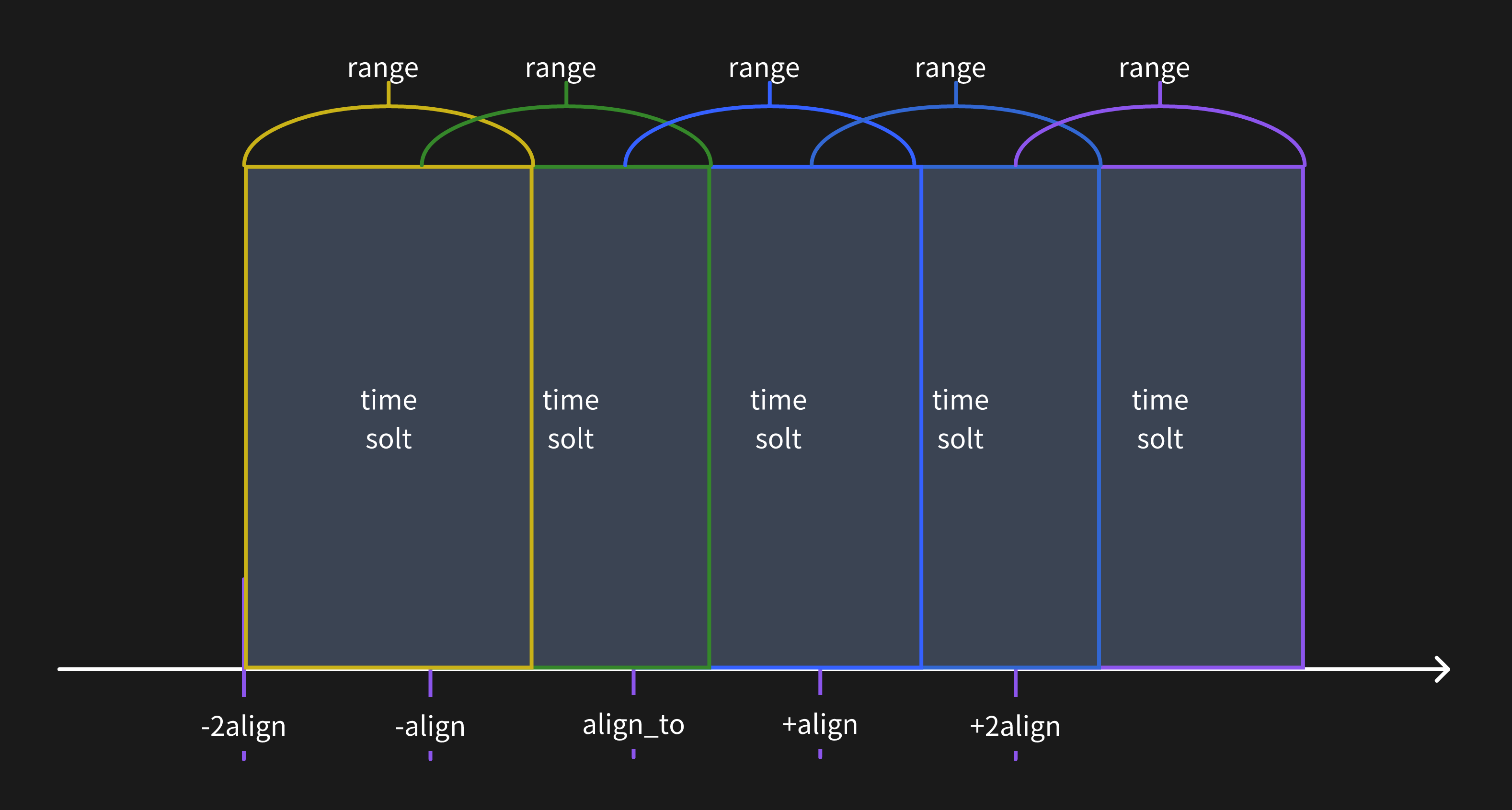
The following images can help you understand the time range window more visually:
When the query resolution is greater than the time range window, the metrics data will be calculated for only one time range window.
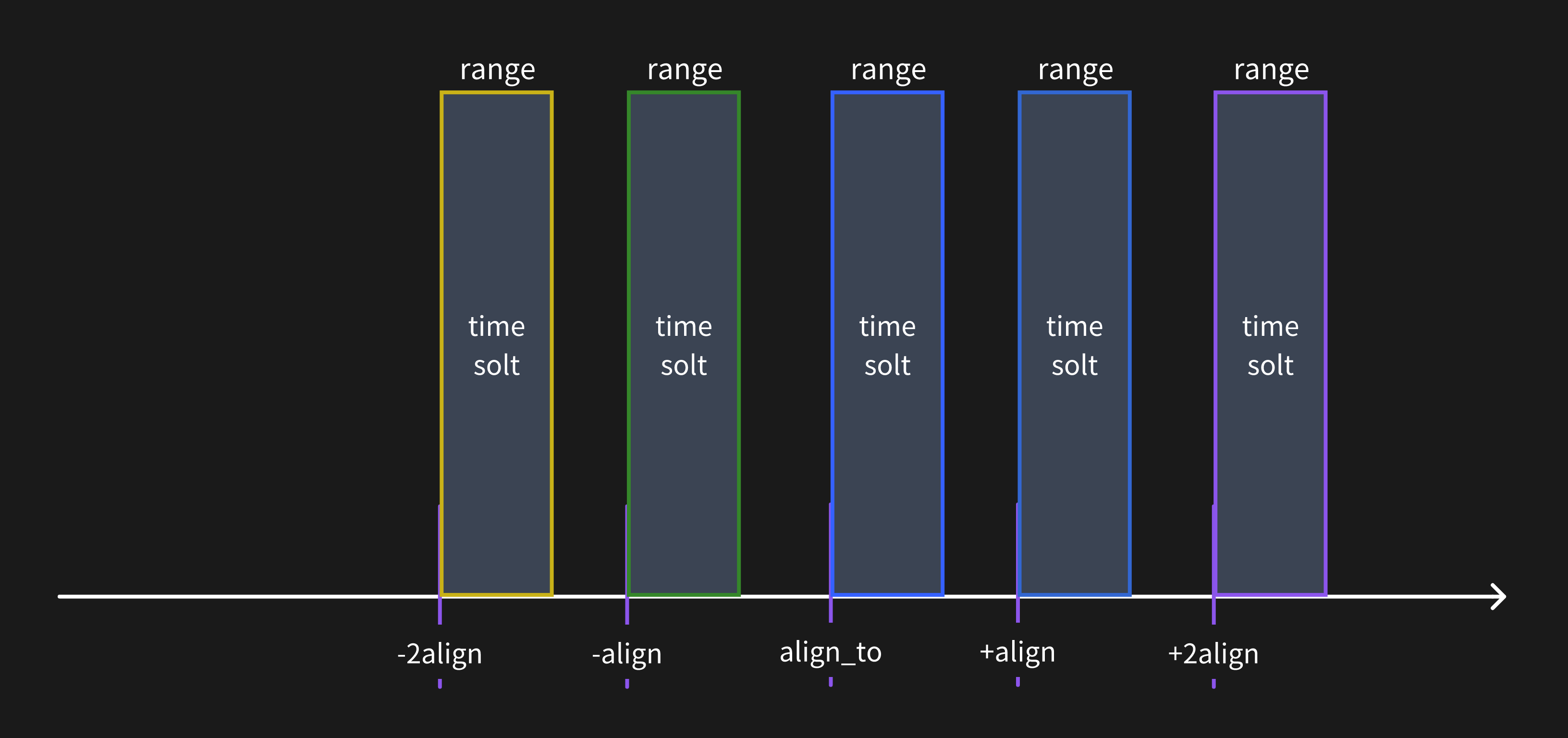
When the query resolution is less than the time range window, the metrics data will be calculated for multiple time range windows.
Align to specific timestamp
The alignment times default based on the time zone of the current SQL client session.
You can change the origin alignment time to any timestamp you want. For example, use NOW to align to the current time:
SELECT
    ts,
    host,
    avg(cpu) RANGE '1w'
FROM monitor
ALIGN '1d' TO NOW BY (host);
Or use a ISO 8601 timestamp to align to a specified time:
SELECT
    ts,
    host,
    avg(cpu) RANGE '1w'
FROM monitor
ALIGN '1d' TO '2023-12-01T00:00:00+08:00' BY (host);
Fill null values
The FILL option can be used to fill null values in the data.
In the above example, the LINEAR method is used to fill null values.
Other methods are also supported, such as PREV and a constant value X.
For more information, please refer to the FILL OPTION.
Syntax
Please refer to Range Query for more information.
Table name constraints
If your table name contains special characters or uppercase letters, you must enclose the table name in backquotes. For examples, please refer to the Table name constraints section in the table creation documentation.
HTTP API
Use POST method to query data:
curl -X POST \
  -H 'authorization: Basic <base64-encoded-credentials>' \
  -H 'Content-Type: application/x-www-form-urlencoded' \
  -d 'sql=select * from monitor' \
http://localhost:4000/v1/sql?db=public
The result is shown below:
{
  "code": 0,
  "output": [
    {
      "records": {
        "schema": {
          "column_schemas": [
            {
              "name": "host",
              "data_type": "String"
            },
            {
              "name": "ts",
              "data_type": "TimestampMillisecond"
            },
            {
              "name": "cpu",
              "data_type": "Float64"
            },
            {
              "name": "memory",
              "data_type": "Float64"
            }
          ]
        },
        "rows": [
          ["127.0.0.1", 1667446797450, 0.1, 0.4],
          ["127.0.0.1", 1667446798450, 0.5, 0.2],
          ["127.0.0.2", 1667446798450, 0.2, 0.3]
        ]
      }
    }
  ],
  "execution_time_ms": 0
}
For more information about SQL HTTP request, please refer to API document.